<?xml version="1.0" encoding="utf-8"?><?xml-stylesheet type="text/xml" href="https://joshua8.ai/feed.xslt.xml"?><feed xmlns="http://www.w3.org/2005/Atom" ><generator uri="https://jekyllrb.com/" version="4.3.4">Jekyll</generator><link href="https://joshua8.ai/feed.xml" rel="self" type="application/atom+xml" /><link href="https://joshua8.ai/" rel="alternate" type="text/html" /><updated>2026-07-04T20:46:57+00:00</updated><id>https://joshua8.ai/feed.xml</id><title type="html">Joshua8.AI</title><subtitle>A founder-led AI venture studio — we build and back AI companies from our own technical and hardware lab.</subtitle><entry><title type="html">What AI Developers Have in Common With Three-Year-Olds on the Boardwalk</title><link href="https://joshua8.ai/two-5070ti-part1-pipeline-vs-tensor-parallel/" rel="alternate" type="text/html" title="What AI Developers Have in Common With Three-Year-Olds on the Boardwalk" /><published>2026-07-03T00:00:00+00:00</published><updated>2026-07-03T00:00:00+00:00</updated><id>https://joshua8.ai/two-5070ti-part1-pipeline-vs-tensor-parallel</id><content type="html" xml:base="https://joshua8.ai/two-5070ti-part1-pipeline-vs-tensor-parallel/"><![CDATA[<p><img src="/images/two-5070ti-part1.png" alt="Two RTX 5070 Tis serving a 35B model — pipeline vs tensor parallelism on consumer Blackwell" /></p>

<p><em>Two 5070 Tis, one 35B model — Part 1 of 3: the parallelism problem (pipeline vs tensor parallel on consumer Blackwell)</em></p>

<h2 id="tldr">TL;DR</h2>

<p>We wanted to serve Qwen3.6-35B-A3B, a 35-billion-parameter mixture-of-experts model, on a desktop with two RTX 5070 Ti cards, 16 GB each. The weights don’t fit on one card, so the model has to be split. The obvious choice, tensor parallelism (TP), turned out to be the wrong one on this hardware: these consumer Blackwell cards have no GPU-to-GPU P2P link, so every layer’s all-reduce crawls over plain PCIe. Pipeline parallelism (PP) splits the model by whole layers, hands off activations only at stage boundaries, and ran prefill <strong>1.9× faster</strong> than TP (~13K vs ~6.8K tok/s). TP won on one axis only (a ~2.5× larger KV cache), but its boot was flaky and its decode was no better. PP became our production split. This post covers <em>why</em> each split behaves the way it does on no-P2P consumer silicon, with the benchmark numbers that settled it.</p>

<hr />

<h2 id="why-run-this-locally-at-all">Why run this locally at all</h2>

<p>Fable 5 shipped, again, and my phone would not stop buzzing. Three developer friends, three separate texts over the course of an afternoon, all some version of the same complaint: <em>out of tokens.</em> Their Claude Max plans had hit the wall on launch day, which is what happens to anything good the moment everyone piles onto it at once.</p>

<p>Then my three-year-old granddaughter walked into the room, planted herself in the doorway, and announced, with total conviction, that <em>she</em> was out of tokens. For a second I thought the outage had achieved sentience. She meant Zelky’s, the arcade down in Rehoboth Beach, where a fistful of tokens buys a fixed amount of whac-a-mole and a few doomed passes at the impossible-to-win stuffed-animal claw, and then, abruptly, does not. Same phrase, same disappointment, entirely different economy. And the only reason she was at the arcade in the first place: her father, the fourth developer of the day, had run out of Claude tokens too, so an afternoon that was supposed to be spent shipping code became an afternoon of whac-a-mole and the claw instead.</p>

<p>The coincidence stuck with me, because a token is a token: a metered unit of something you want more of than you’re given. When the good model ships and everyone shows up, the shared meter runs dry, for a developer on a Max plan and a three-year-old at a claw machine alike. The way out is to own the machine that mints them. Two consumer GPUs and a decent open-weight 35B model, and the meter is yours: no per-request billing, no launch-day rate limit, no afternoon of “out of tokens” texts. The arcade doesn’t run out when you own the arcade.</p>

<p>That’s the motivation. The rest of this series is what it took to get a genuinely useful open-weight model (not frontier-class, but more than good enough for real work) running on hardware you can buy at Walmart. It wasn’t free either; the currency was three weeks of debugging instead of dollars. Here’s how it went.</p>

<h2 id="the-box">The box</h2>

<p>The machine is deliberately unglamorous: two NVIDIA RTX 5070 Ti GPUs, Blackwell architecture, compute capability 12.0 (SM120), 16 GB of VRAM each, hanging off a consumer Intel Core Ultra 9 on a consumer motherboard. Not an H100 with NVLink. Not a workstation board with two full-width slots wired for P2P. This is a gaming desktop pressed into service as an inference server, and its interconnect topology shows it.</p>

<p>Look at how the two cards are actually attached. The board has exactly one PCIe 5.0 x16 slot, and that’s where card 0 lives, with a proper fat pipe to the CPU. There’s nowhere on the board to put a second card at anything like that width. So card 1 is hung off an Oculink cable running PCIe 4.0 x4. Do the arithmetic on that link: PCIe 4.0 x4 is ~8 GB/s in each direction, roughly an eighth of the x16 5.0 slot the other card enjoys, and a rounding error next to the ~450 GB/s of an NVLink bridge. The two GPUs aren’t just missing a fast link between them; the <em>second card’s link to the rest of the machine is a drinking straw.</em></p>

<p>And it gets worse for the thing TP needs most: on this consumer platform the GPUs cannot DMA directly into each other’s memory. There is no P2P path. Anything one card needs from the other doesn’t even get the straw directly. It rides <em>up</em> card 1’s PCIe 4.0 x4 Oculink link to the CPU’s root complex and <em>back down</em> card 0’s link, a full host bounce, on top of the width mismatch.</p>

<p>That combination — no P2P, and an asymmetric x16 / x4 topology — ends up dictating almost every architectural decision in this series. Any strategy that chats constantly between the cards is paying tolls at the slowest link on the board.</p>

<p>The model is Qwen3.6-35B-A3B: 35B total parameters, but a mixture-of-experts design that activates only ~3B per token (the “A3B”). It’s also a <em>hybrid</em> model: it interleaves Gated Delta Net (GDN) linear-attention layers with full-attention layers, which matters enormously later. In INT4 (Intel AutoRound) the weights are ~13.5 GB; in native FP4 (NVFP4) they’re ~22 GB. Either way, one 16 GB card can’t hold the whole thing plus a usable KV cache plus activation scratch. It must be split.</p>

<h2 id="two-ways-to-split-a-model">Two ways to split a model</h2>

<p>There are two standard ways to shard a transformer across GPUs:</p>

<p><strong>Tensor parallelism (TP)</strong> slices <em>every</em> weight matrix across cards: each GPU holds half of every layer’s columns/rows. To compute a single layer you must combine partial results from both cards with an all-reduce. That’s a collective communication on <em>every layer, every forward pass</em>. TP is the darling of datacenter deployments precisely because NVLink makes those all-reduces nearly free.</p>

<p><strong>Pipeline parallelism (PP)</strong> slices the model by <em>depth</em>: card 0 holds the first N layers, card 1 holds the rest. Activations cross the PCIe bus exactly once per micro-batch, at the single stage boundary. No per-layer collective. The cost is “pipeline bubble”: while card 1 works on the back half, card 0 could be idle unless you keep multiple micro-batches in flight.</p>

<p>On NVLink hardware, TP usually wins. The received wisdom is “use TP within a node, PP across nodes.” We are inside a node, so TP should win here too, right?</p>

<p>It didn’t, for three reasons that all trace back to that interconnect.</p>

<h2 id="why-tp-loses-on-no-p2p-consumer-cards">Why TP loses on no-P2P consumer cards</h2>

<p>Three separate failure modes stacked up against TP on this box.</p>

<p><strong>1. The all-reduce tax over a x4 host bounce.</strong> With no P2P, every per-layer all-reduce is a round trip through host memory, and its throughput is gated by the <em>slowest</em> link in the path, which on this board is card 1’s PCIe 4.0 x4 Oculink straw (~8 GB/s). Qwen3.6 has dozens of layers; at TP=2 you pay two of those collectives (one for attention, one for the MLP) <em>per layer, per token batch</em>, each one squeezing through that x4 pipe and bouncing off the CPU. On NVLink that’s tens of microseconds; over an x4 host bounce it’s an order of magnitude worse, and it lands directly on the prefill critical path. This is the dominant reason TP prefill came in at roughly half PP’s throughput. PP, by contrast, crosses that slow link <em>once per micro-batch</em> at the single stage boundary instead of twice per layer. It’s the one strategy that respects the drinking straw.</p>

<p><strong>2. Marlin’s minimum tile width.</strong> The FP4/INT4 dense linear layers fall back to the Marlin GEMM kernel, which has a hard <code class="language-plaintext highlighter-rouge">min_thread_n = 64</code> — the output dimension of a sharded matmul can’t go below 64 columns. TP=2 slices those dense layers in half; several of them drop under Marlin’s floor and the model simply fails to load. PP never slices a matrix — it moves whole layers — so nothing ever falls under the kernel’s minimum. (This bit us specifically on the NVFP4 build, covered in Part 2.)</p>

<p><strong>3. The vision tower gets replicated.</strong> Qwen3.6 is multimodal — it ships a BF16 vision transformer (ViT) for image inputs. Under TP the ViT is <em>replicated on every card</em>, so an image request inflates memory symmetrically on both GPUs and OOMs them together. Under PP the ViT runs on rank 0 only. On 16 GB cards already ~85% full of weights, that replicated ViT is the difference between “images work” and “engine dies.” (Part 3 is entirely about attacking this problem from the other side — evicting the ViT from the GPU altogether.)</p>

<p>None of these three is fatal <em>alone</em>. Together they make TP the wrong default on this hardware.</p>

<h2 id="the-one-thing-tp-is-genuinely-better-at">The one thing TP is genuinely better at</h2>

<p>TP isn’t strictly worse. It has a real, measurable advantage: KV cache capacity.</p>

<p>Because TP shards the weights <em>and</em> the per-layer activation working set across both cards, each GPU carries a lighter fixed load, and the memory the profiler can hand to the paged KV cache roughly doubles. On the GDN hybrid layers, TP also halves the linear-attention state each card must hold. Concretely, at the same context length:</p>

<table>
  <thead>
    <tr>
      <th>Split</th>
      <th style="text-align: right">KV cache pool</th>
      <th style="text-align: right">Relative</th>
      <th style="text-align: right">Prefill throughput</th>
      <th style="text-align: right">Decode</th>
      <th>Boot reliability</th>
    </tr>
  </thead>
  <tbody>
    <tr>
      <td><strong>PP=2</strong></td>
      <td style="text-align: right">196,608 tok</td>
      <td style="text-align: right">1.00×</td>
      <td style="text-align: right"><strong>~12.8–13.5K tok/s</strong></td>
      <td style="text-align: right">baseline</td>
      <td>reliable</td>
    </tr>
    <tr>
      <td><strong>TP=2</strong></td>
      <td style="text-align: right">~503,316 tok</td>
      <td style="text-align: right"><strong>2.56×</strong></td>
      <td style="text-align: right">~6.7–6.8K tok/s</td>
      <td style="text-align: right">≤ PP at every N</td>
      <td><strong>flaky (2/3 boots died)</strong></td>
    </tr>
  </tbody>
</table>

<p>So if your workload is <em>text-only, high-concurrency, very-long-context</em>, the regime where you’re starved for KV pages and don’t care about prefill latency, TP’s 2.5× bigger cache could be the deciding factor. That’s a real niche. It just isn’t <em>our</em> niche.</p>

<h2 id="the-flaky-boot-problem">The flaky-boot problem</h2>

<p>TP had one more strike that doesn’t show up in a throughput table: it wouldn’t boot reliably. Roughly two out of every three cold starts hung silently in NCCL rendezvous — the two ranks never completed their handshake, no error, just a process sitting forever at initialization. A retry loop and <code class="language-plaintext highlighter-rouge">--force-recreate</code> got it up eventually, but “eventually, after two silent hangs” is not a property you want in a service that’s supposed to <code class="language-plaintext highlighter-rouge">restart: unless-stopped</code>. PP boots cleanly, first try, essentially every time.</p>

<p>We never fully root-caused the rendezvous hangs — on a two-GPU single-host setup they’re most likely a shared-memory/IPC timing issue in the collective bootstrap, aggravated by the no-P2P topology. For a production decision it didn’t matter: unreliable boot was disqualifying on its own.</p>

<h2 id="reading-the-throughput-numbers">Reading the throughput numbers</h2>

<p>The prefill gap is worth staring at, because it’s bigger than most people expect. ~13K vs ~6.8K tok/s isn’t a rounding difference — it’s TP paying the PCIe all-reduce tax on a workload that is <em>dominated by prefill</em>. When you feed a long prompt, the model runs one big parallel forward over all prompt tokens; that’s exactly where TP’s per-layer collectives pile up and PP’s single boundary hand-off shines.</p>

<p>Decode (token-by-token generation) is a different story — it’s memory-bandwidth-bound per card and the communication is a smaller fraction of the step, so PP and TP land close. But PP was ≥ TP at every concurrency level we measured, so there was no decode-side reason to prefer TP either.</p>

<p>One measurement caveat that cost us real debugging time: the GDN hybrid layers JIT-compile a CuteDSL kernel that recompiles whenever the request <em>shape</em> changes sharply (a big prefill followed by a small decode). The first small request after a large one can eat an ~8–17 second engine stall, and if you’re not careful you’ll measure that stall as “decode throughput” and get ~113 tok/s when the warm number is ~171. We learned to run best-of-N warm timings. We dig into that stall in Part 2, because on the NVFP4 build it got much worse.</p>

<h2 id="the-kv-cache-paradox-why-16-concurrent-sequences-fit-in-a-pool-that-cant-hold-them">The KV-cache paradox: why 16 concurrent sequences fit in a pool that “can’t hold them”</h2>

<p>There’s a number that looks alarming until you understand vLLM’s scheduler. At 196,608 tokens of context and 16 concurrent sequences, a naive reading says you need 16 × 196,608 ≈ 3.1M tokens of KV cache to guarantee every sequence its full context. Our pool is 196,608 tokens — <em>one</em> sequence’s worth. By that arithmetic the server should fall over the moment two long requests arrive.</p>

<p>It doesn’t, because vLLM’s V1 scheduler is admit-and-queue, not admit-and-preempt. It doesn’t promise every admitted sequence its maximum context up front; it pages KV in as tokens are actually generated, and when the pool gets tight it <em>queues</em> waiting sequences rather than evicting running ones. Under a deliberate 16-way stress test we watched the scheduler settle at ~7 running, 11 waiting, KV at 88.8% utilization, and zero preemptions. The structural preemption trigger (the one that would thrash) turned out to be unreachable for this configuration. Real prompts don’t all demand full context simultaneously; the pool is sized for the <em>working set</em>, not the theoretical worst case.</p>

<p>This matters for the PP-vs-TP decision because it defuses TP’s one advantage. TP’s 2.5× bigger pool sounds decisive only if you believe you need pool ≈ seqs × context. You don’t. Once the scheduler is doing its job, a 196,608-token pool comfortably serves 16 concurrent sequences at long context — so PP’s smaller pool stops being a liability, and its prefill speed and clean boot carry the decision unopposed.</p>

<h2 id="what-prefill-heavy-actually-means-for-the-split">What “prefill-heavy” actually means for the split</h2>

<p>One more piece of context makes the PP choice concrete rather than abstract. Our workload is <em>prefill-heavy</em>: long prompts (documents, long chat histories, images that expand into thousands of vision tokens) relative to the number of tokens generated back. That’s the regime where the forward pass over the prompt dominates wall-clock, and it’s exactly the regime where TP’s per-layer all-reduce tax is most punishing and PP’s single boundary hand-off is cheapest.</p>

<p>If the workload were the opposite — short prompts, long generations, dozens of concurrent streams all starved for KV pages — the calculus would shift toward TP’s bigger pool and away from PP’s prefill edge. We didn’t have that workload. But because we <em>built and validated</em> the TP path anyway (Part 3 shows how), switching is a config change, not a re-architecture, if the traffic ever inverts.</p>

<h2 id="why-this-ordering-of-evidence-matters">Why this ordering of evidence matters</h2>

<p>The takeaway isn’t “PP good, TP bad.” It’s that the right parallelism strategy is a property of your interconnect and your workload, not a universal ranking. On an NVLink DGX, TP=2 for this model would likely win outright. On two consumer cards with no P2P, serving a prefill-heavy multimodal workload, PP wins on throughput, boots reliably, and keeps the vision tower on a single card. TP keeps exactly one trophy, KV capacity, that we didn’t need.</p>

<p>So production runs <strong>PP=2</strong>: 196,608-token context, the vision tower native on rank 0, both cards ~85–92% utilized, clean boots. That’s the split.</p>

<p>But settling PP vs TP was the <em>easy</em> half. The hard half was getting the native-FP4 build to produce correct text at all — which meant bisecting nine days of vLLM nightlies to find the one that didn’t output garbage, and diagnosing an SM120 kernel crash that only exists on consumer Blackwell. That’s Part 2.</p>

<hr />

<p><em>Next — Part 2, “The Nightly From Hell”: bisecting vLLM to find a working NVFP4 build, and the SM120 FP4 crash nobody documents.</em></p>]]></content><author><name>Jim Smith</name></author><category term="AI Technology" /><category term="vllm" /><category term="qwen" /><category term="pipeline-parallel" /><category term="tensor-parallel" /><category term="blackwell" /><category term="5070ti" /><category term="local-llm" /><category term="moe" /><summary type="html"><![CDATA[Two RTX 5070 Tis, one 35B MoE model. Why pipeline parallelism beat tensor parallelism 1.9x on prefill on consumer Blackwell cards with no GPU-to-GPU P2P link.]]></summary></entry><entry><title type="html">200 Billion Parameters for $1,000: Running 4-Bit Quants on eBay Hardware</title><link href="https://joshua8.ai/200b-parameters-1000-ebay-hardware/" rel="alternate" type="text/html" title="200 Billion Parameters for $1,000: Running 4-Bit Quants on eBay Hardware" /><published>2026-06-21T00:00:00+00:00</published><updated>2026-06-21T00:00:00+00:00</updated><id>https://joshua8.ai/200b-parameters-1000-ebay-hardware</id><content type="html" xml:base="https://joshua8.ai/200b-parameters-1000-ebay-hardware/"><![CDATA[<p><img src="/images/200b-ebay-hardware.png" alt="200 billion parameters for $1,000 — running large MoE models on budget eBay hardware" /></p>

<p><strong>TL;DR</strong>
You can run frontier-size mixture-of-experts (MoE) models—such as Qwen3.5-122B, MiniMax-M2.7 (~229B), and DeepSeek-V4-Flash (284B)—on a modest GPU backed by standard system RAM using <code class="language-plaintext highlighter-rouge">llama.cpp</code>’s <code class="language-plaintext highlighter-rouge">--cpu-moe</code> flag. This works because these models only activate a fraction of their parameters per token (around 10–13B), allowing the massive “expert” weights to live in cheap system RAM while the GPU handles attention and the KV cache.</p>

<p>While a $12.5K RTX PRO 6000 setup runs Qwen3.5-122B at a blistering 128 tokens per second (tok/s) for a single user—and an aggregate 780 tok/s for a concurrency of 8 users—a $1,000 eBay-scavenged Xeon workstation with 2016-era Pascal cards runs the same model at ~10 tok/s. It’s slower, yes, but still faster than most people read—and entirely usable for a single person. You sacrifice raw concurrency, not capability.</p>

<hr />

<p>The prevailing advice for running massive MoE models locally usually demands a massive budget: drop $25,000 on two RTX PRO 6000 Blackwells, buy two DGX Sparks (which run about $4,699 each), or pick up two Strix Halos with 128GB of unified memory (priced around $3,999 each). The logic assumes that because 4-bit model weights take up 70–160GB, you need a matching mountain of ultra-fast VRAM.</p>

<p>You don’t.</p>

<p>Over the past two weeks, I’ve been running Qwen3.5-122B-A10B, MiniMax-M2.7 (~229B), and DeepSeek-V4-Flash (284B) on setups that look nothing like a datacenter. One is a machine with a single RTX 5090, and the other is a ~$1,000 workstation built from eBay parts featuring a pair of $250 Quadro P5000s from 2016. The secret lies in a <code class="language-plaintext highlighter-rouge">llama.cpp</code> feature called <code class="language-plaintext highlighter-rouge">--cpu-moe</code>, which exploits a massive architectural asymmetry that standard hardware advice ignores.</p>

<h2 id="the-fact-that-changes-the-math">The Fact That Changes the Math</h2>

<p>Running a dense 122B model on a CPU would be agonizing. Every generated token requires touching all 122 billion parameters. Because CPU memory bandwidth (a few hundred GB/s on DDR4/DDR5) is an order of magnitude slower than a GPU, you would wait seconds for a single token.</p>

<p>But new MoE models aren’t dense. Consider the active parameters:</p>

<ul>
  <li><strong>Qwen3.5-122B-A10B:</strong> 122B total, 10B active per token.</li>
  <li><strong>MiniMax-M2.7:</strong> 229B total, ~10B active per token.</li>
  <li><strong>DeepSeek-V4-Flash:</strong> 284B total, 13B active per token.</li>
</ul>

<p>This asymmetry changes everything. The bulk of the weights—tens of gigabytes of “experts”—sit idle for any given token. Using the <code class="language-plaintext highlighter-rouge">--cpu-moe</code> (or <code class="language-plaintext highlighter-rouge">-cmoe</code>) flag stores these mostly dormant experts in affordable system RAM. Only the components that touch <em>every</em> token—the attention layers, dense projections, and KV cache—remain on the GPU.</p>

<p>The result is a clean division of labor: the modest GPU handles the compute-intensive attention math, while cheap system RAM holds the massive pile of sleeping experts.</p>

<h2 id="the-two-budget-boxes">The Two Budget Boxes</h2>

<ul>
  <li><strong>The Ryzen Box:</strong> A more conventional build pairing an RTX 5090 (32GB, Blackwell) with an AMD Ryzen 9 9950X (16 cores / 32 threads) and 192GB of DDR5 RAM. The total build costs about $5,000, which includes the ~$3,200 GPU.</li>
  <li><strong>The Xeon Box:</strong> Built purely from older eBay parts, featuring dual Intel Xeon E5-2698 v4 CPUs (2016 Broadwell, 40 physical cores total), 128GB of DDR4 RAM, and two Quadro P5000s (16GB VRAM each). The GPUs were $250 each, the CPUs were $100 for the pair, and the chassis/board/RAM cost $425. Total cost: ~$1,000 for 32GB of aggregate VRAM and enough system memory to host a 108GB model.</li>
</ul>

<p><em>(Note: These prices are roughly a year old, sourced before recent DRAM spikes. Replicating the $1,000 box today might cost closer to $1,400–$1,800 due to memory pricing.)</em></p>

<h2 id="the-performance-numbers">The Performance Numbers</h2>

<p>Here is the single-stream decode throughput for Qwen3.5-122B-A10B, comparing our budget boxes against a “money-no-object” $12.5K RTX PRO 6000 reference machine:</p>

<table>
  <thead>
    <tr>
      <th>Machine</th>
      <th>GPU(s)</th>
      <th>Total Box Cost</th>
      <th>Decode Speed</th>
    </tr>
  </thead>
  <tbody>
    <tr>
      <td>RTX PRO 6000</td>
      <td>1× Blackwell 96GB</td>
      <td>~$12.5K</td>
      <td>128 tok/s</td>
    </tr>
    <tr>
      <td>Ryzen Box</td>
      <td>1× RTX 5090 32GB</td>
      <td>~$5,000</td>
      <td>22.8 tok/s</td>
    </tr>
    <tr>
      <td>Xeon Box</td>
      <td>2× Pascal P5000 16GB</td>
      <td>~$1,000</td>
      <td>~10 tok/s</td>
    </tr>
  </tbody>
</table>

<p>The $12.5K setup (a $10K card and a $2.5K box) is instantly responsive because it holds all 73GB of quantized weights in VRAM. But a $1,000 box with nine-year-old GPUs running a 122-billion-parameter model at 10 tokens per second is highly usable for interactive chat or coding assistance.</p>

<p>The Ryzen box is roughly twice as fast as the Xeon for two reasons—and the first one is easy to get backwards. With <code class="language-plaintext highlighter-rouge">--cpu-moe</code>, the experts that dominate decode are streamed from <em>system</em> RAM, not from the GPU. The Ryzen’s DDR5 is considerably faster than the Xeon’s 2016-era DDR4, so the host memory feeding those experts is the real difference. (The 5090’s own GDDR7 VRAM is faster still, but the offloaded experts never live there—only the attention layers and KV cache do.) Second, the modern 5090 chews through the attention math far quicker than a pair of Pascal P5000s.</p>

<h2 id="the-trade-offs-of-cpu-offloading">The Trade-offs of CPU Offloading</h2>

<p>This approach isn’t free. Here are the very real bottlenecks:</p>

<ul>
  <li><strong>Decode is CPU-bandwidth-bound:</strong> The speed limit (10–23 tok/s) is dictated by how fast your RAM feeds the active experts to the CPU cores. Relying on hyperthreading can actually hurt performance; sticking to physical cores yields better results.</li>
  <li><strong>Prefill is compute-bound and agonizingly slow:</strong> Digesting a long prompt requires raw FLOPS and TOPS, which old CPUs severely lack.</li>
  <li><strong>Context is surprisingly cheap:</strong> Because the massive experts live in RAM, your GPU effortlessly handles the KV cache. The RTX 5090 fits Qwen3.5-122B’s entire 256K context into just 12GB of VRAM.</li>
  <li><strong>You must pin the experts in RAM:</strong> Using <code class="language-plaintext highlighter-rouge">--no-mmap</code> and <code class="language-plaintext highlighter-rouge">--mlock</code> together prevents the kernel from paging files out to swap memory mid-generation.</li>
</ul>

<h2 id="the-asymmetry-prefill-vs-generation">The Asymmetry: Prefill vs. Generation</h2>

<p>An LLM request has two phases with entirely different bottlenecks. <strong>Generation</strong> is memory-bandwidth-bound, but <strong>prefill</strong> (digesting the prompt) is compute-bound.</p>

<p>While the dual Xeon’s 150 GB/s memory bandwidth is about 10% of the RTX PRO 6000’s 1.8 TB/s, the compute gap is astronomical. The Blackwell card delivers 125 TFLOPS of FP32 and 4,000 AI TOPS via tensor cores, whereas the 2016 Xeons manage only ~2.8 TFLOPS of FP32 with zero tensor cores.</p>

<p>The rule of thumb: decode speed barely moves with prompt length, but prefill cost explodes. A 44.5K token prefill for DeepSeek-V4-Flash took roughly 10 minutes on the Ryzen box. Extrapolating a 256K-token prompt implies waiting over an hour just for the first token. <strong>Pick your hardware by your expected prompt length, not just your model size.</strong></p>

<h2 id="concurrency-what-the-125k-box-actually-buys">Concurrency: What the $12.5K Box Actually Buys</h2>

<p>When serving Qwen3.5-122B via vLLM on the RTX PRO 6000, a single user gets 128 tok/s, but pushing a concurrency of 8 users yields a massive 780 tok/s aggregate throughput.</p>

<p>CPU-offloading cannot match this. On the 5090, pushing multiple requests causes aggregate throughput to rise sub-linearly, while the per-request rate collapses from 23 tok/s to roughly 8.5 tok/s as the CPU experts saturate. If you need to serve a team, buy the big card.</p>

<h2 id="important-caveats--setup">Important Caveats &amp; Setup</h2>

<ul>
  <li><strong>Old GPUs mean old CUDA:</strong> The P5000s are Pascal architecture, meaning they are pinned to a CUDA-12.8 <code class="language-plaintext highlighter-rouge">llama.cpp</code> image since CUDA 13 dropped Pascal support.</li>
  <li><strong>DeepSeek-V4-Flash:</strong> This architecture requires a community fork to run properly, so verified numbers are only available for the Ryzen box (hitting 11–12 tok/s).</li>
  <li><strong>Heat and Power Draw:</strong> Old servers are power hungry. The small server room holding the boxes for these tests rose to 83°F when I started running these evals—just a bit too warm for the office. Expect about 800W of power draw on the dual Xeons, and pushing 1000W+ on the RTX 5090 setup.</li>
</ul>

<p><strong>The Flags You Need</strong>:</p>

<ul>
  <li><code class="language-plaintext highlighter-rouge">--cpu-moe</code> (or <code class="language-plaintext highlighter-rouge">--n-cpu-moe N</code> to shift layers manually).</li>
  <li><code class="language-plaintext highlighter-rouge">--no-mmap</code> and <code class="language-plaintext highlighter-rouge">--mlock</code> to pin weights in anonymous RAM. On the Ryzen box, MiniMax’s 131GB pins cleanly into the 192GB of RAM; on the Xeon, an IQ4_XS quant’s ~108GB pin leaves about ~20GB free on the 128GB box.</li>
  <li><code class="language-plaintext highlighter-rouge">--flash-attn on</code> alongside a quantized KV cache (like <code class="language-plaintext highlighter-rouge">q8_0</code>) to save VRAM.</li>
  <li><code class="language-plaintext highlighter-rouge">--threads</code> set strictly to physical cores (plus <code class="language-plaintext highlighter-rouge">--numa distribute</code> for dual-socket setups).</li>
  <li><code class="language-plaintext highlighter-rouge">--parallel 1</code> to dedicate the entire context window to a single user.</li>
</ul>

<h2 id="conclusion">Conclusion</h2>

<p>This was never about speed; it’s about access. You are giving up the headroom for concurrency and the instant first token. But you are gaining the ability to run 122-billion, 229-billion, or 284-billion-parameter models on hardware that costs as much as a used laptop.</p>]]></content><author><name>Jim Smith</name></author><category term="AI Technology" /><category term="llama-cpp" /><category term="qwen" /><category term="minimax" /><category term="deepseek" /><category term="moe" /><category term="cpu-offload" /><category term="local-llm" /><category term="pascal" /><category term="rtx-5090" /><category term="budget" /><summary type="html"><![CDATA[How I run Qwen3.5-122B, MiniMax-M2.7, and DeepSeek-V4-Flash on a modest GPU (15-32GB VRAM) plus cheap CPU RAM using llama.cpp's --cpu-moe expert offload. Benchmarks from an RTX 5090 box and a $1,000 eBay Xeon.]]></summary></entry><entry><title type="html">Revisiting LegalBench: New Models, A Bug I Missed, and a New Leader</title><link href="https://joshua8.ai/legalbench-revisited-new-models-bug-fix/" rel="alternate" type="text/html" title="Revisiting LegalBench: New Models, A Bug I Missed, and a New Leader" /><published>2026-04-17T00:00:00+00:00</published><updated>2026-04-17T00:00:00+00:00</updated><id>https://joshua8.ai/legalbench-revisited-new-models-bug-fix</id><content type="html" xml:base="https://joshua8.ai/legalbench-revisited-new-models-bug-fix/"><![CDATA[<p><img src="/images/legalbench-revisited.png" alt="LegalBench revisited — new models, bug fix, and a new leader" /></p>

<p>Last month I published <a href="/legalbench-smaller-ai-beats-bigger-at-law/">benchmark results</a> comparing five LLMs on LegalBench, a suite of 161 legal reasoning tasks. The 27B Qwen3.5 model won at 0.7936, beating a 120B reasoning model by 6 points. The headline was that bigger isn’t better for legal work.</p>

<p>Since then, two things happened. First, I added two more models to the lineup: Qwen3.6-35B (which dropped yesterday) and Qwen3.5-122B (which I simply didn’t evaluate in round one). Second, I found a bug in my benchmarking code that was quietly suppressing scores on one category of tasks. Fixing it changes the leaderboard.</p>

<h2 id="the-additional-models">The Additional Models</h2>

<p>Both are MoE architectures from the Qwen team:</p>

<table>
  <thead>
    <tr>
      <th>Model</th>
      <th>Total params</th>
      <th>Active params</th>
      <th>Quantization</th>
    </tr>
  </thead>
  <tbody>
    <tr>
      <td>Qwen3.6-35B</td>
      <td>35B</td>
      <td>~3B (A3B)</td>
      <td>AWQ 4-bit</td>
    </tr>
    <tr>
      <td>Qwen3.5-122B</td>
      <td>122B</td>
      <td>~10B (A10B)</td>
      <td>AWQ 4-bit</td>
    </tr>
  </tbody>
</table>

<p>Both AWQ 4-bit quantizations were produced by <a href="https://huggingface.co/cyankiwi">cyankiwi</a>. The 3.6-35B ran on my RTX 5090; the 122B ran on an RTX 6000 Pro. Both served via vLLM in no-think mode, same prompts as the original benchmark.</p>

<h2 id="the-bug-i-missed">The Bug I Missed</h2>

<p>When I pulled the raw outputs for the MAUD category — 34 tasks on M&amp;A agreement interpretation that use A/B/C/D/E multiple-choice — I noticed something weird. Qwen3.6-35B had scored <strong>0.012</strong> on <code class="language-plaintext highlighter-rouge">maud_fiduciary_exception_board_determination_trigger_(no_shop)</code>. That’s below random chance for a binary question.</p>

<p>A look at the generations explained it: the model was answering <code class="language-plaintext highlighter-rouge">"Option B"</code> while the gold label was <code class="language-plaintext highlighter-rouge">"B"</code>. My <code class="language-plaintext highlighter-rouge">extract_answer()</code> function was returning the full string <code class="language-plaintext highlighter-rouge">"Option B"</code>, which never matched <code class="language-plaintext highlighter-rouge">"B"</code> in the grader.</p>

<p>Worse, on some tasks the model answered <code class="language-plaintext highlighter-rouge">"Yes"</code> when the question was A/B multiple choice. The “disproportionate impact modifier” prompts read like yes/no questions, and the model took the bait.</p>

<p>This was present in every model’s results to varying degrees:</p>

<table>
  <thead>
    <tr>
      <th>Model</th>
      <th>MAUD tasks affected</th>
    </tr>
  </thead>
  <tbody>
    <tr>
      <td>Nemotron-30B</td>
      <td>15</td>
    </tr>
    <tr>
      <td>Qwen3.6-35B</td>
      <td>20</td>
    </tr>
    <tr>
      <td>Qwen3.5-35B</td>
      <td>6</td>
    </tr>
    <tr>
      <td>gpt-oss-120b</td>
      <td>4</td>
    </tr>
    <tr>
      <td>Qwen3.5-27B</td>
      <td>4</td>
    </tr>
    <tr>
      <td>Qwen3.5-9B</td>
      <td>2</td>
    </tr>
    <tr>
      <td>Qwen3.5-122B</td>
      <td>0</td>
    </tr>
  </tbody>
</table>

<p>The 122B got clean letters on everything — the issue was specific to how smaller models handled the MAUD prompt format. Still, a benchmark bug is a benchmark bug.</p>

<h2 id="the-fix">The Fix</h2>

<p>Two changes to <code class="language-plaintext highlighter-rouge">run_legalbench.py</code>:</p>

<ol>
  <li><strong>Output extraction</strong> — added a regex to strip <code class="language-plaintext highlighter-rouge">"Option X"</code> prefix: <code class="language-plaintext highlighter-rouge">^Option\s+([A-Z])\b → \1</code></li>
  <li><strong>System prompt</strong> — added an explicit instruction: “If the question offers lettered answer choices (A, B, C, …), reply with ONLY the letter — never ‘Yes’ or ‘No’, never ‘Option X’, just the letter.”</li>
</ol>

<p>I re-ran the 20 problematic MAUD tasks for Qwen3.6-35B with both fixes in place. The results were dramatic:</p>

<table>
  <thead>
    <tr>
      <th>Task</th>
      <th>Before</th>
      <th>After</th>
      <th>Delta</th>
    </tr>
  </thead>
  <tbody>
    <tr>
      <td>fiduciary_exception_board_determination_trigger</td>
      <td>0.012</td>
      <td>0.964</td>
      <td><strong>+0.952</strong></td>
    </tr>
    <tr>
      <td>specific_performance</td>
      <td>0.317</td>
      <td>0.994</td>
      <td>+0.677</td>
    </tr>
    <tr>
      <td>pandemic_or_other_public_health_event (disproportionate)</td>
      <td>0.025</td>
      <td>0.650</td>
      <td>+0.625</td>
    </tr>
    <tr>
      <td>ordinary_course_efforts_standard</td>
      <td>0.325</td>
      <td>0.933</td>
      <td>+0.608</td>
    </tr>
    <tr>
      <td>cor_standard_(intervening_event)</td>
      <td>0.183</td>
      <td>0.762</td>
      <td>+0.579</td>
    </tr>
    <tr>
      <td>general_economic_and_financial_conditions</td>
      <td>0.006</td>
      <td>0.524</td>
      <td>+0.518</td>
    </tr>
    <tr>
      <td>(15 others)</td>
      <td>…</td>
      <td>…</td>
      <td>+0.12 to +0.45</td>
    </tr>
  </tbody>
</table>

<p>Every one of the 20 tasks improved. No regressions. Qwen3.6-35B’s overall score went from <strong>0.7483 to 0.7982</strong> — a +5.0 point jump from an extraction fix alone.</p>

<p>I didn’t re-run the fix on the other models. Their rankings in the original post stand, but be aware that Nemotron and the older 35B are underreported. If I re-ran Nemotron with the fix, I’d expect it to gain 5-8 points and climb out of last place.</p>

<h2 id="updated-leaderboard">Updated Leaderboard</h2>

<table>
  <thead>
    <tr>
      <th>Rank</th>
      <th>Model</th>
      <th>Score</th>
      <th>Notes</th>
    </tr>
  </thead>
  <tbody>
    <tr>
      <td>1</td>
      <td><strong>Qwen3.5-122B</strong></td>
      <td><strong>0.7990</strong></td>
      <td>MoE, 10B active</td>
    </tr>
    <tr>
      <td>2</td>
      <td>Qwen3.6-35B</td>
      <td>0.7982</td>
      <td>MoE, 3B active — after MAUD fix</td>
    </tr>
    <tr>
      <td>3</td>
      <td>Qwen3.5-27B</td>
      <td>0.7936</td>
      <td>Dense</td>
    </tr>
    <tr>
      <td>4</td>
      <td>Qwen3.5-35B</td>
      <td>0.7612</td>
      <td>MoE, 3B active</td>
    </tr>
    <tr>
      <td>5</td>
      <td>Qwen3.5-9B</td>
      <td>0.7583</td>
      <td>Dense</td>
    </tr>
    <tr>
      <td>6</td>
      <td>gpt-oss-120b</td>
      <td>0.7313</td>
      <td>Reasoning model</td>
    </tr>
    <tr>
      <td>7</td>
      <td>Nemotron-30B</td>
      <td>0.5509</td>
      <td>MoE (would gain ~5-8 pts with fix)</td>
    </tr>
  </tbody>
</table>

<p>The top three models are separated by less than one point. The 122B edges out the 3.6-35B by 0.0008 — statistical noise.</p>

<h2 id="what-the-122b-buys-you">What the 122B Buys You</h2>

<p>The 122B has 3.5x more total parameters than the 3.6-35B and runs with 3.3x more active parameters per token. For a one-point gain over the 3.6-35B, is it worth it?</p>

<p>Looking at head-to-head on the 34 MAUD tasks (where the 122B should theoretically benefit most from its extra capacity):</p>

<table>
  <thead>
    <tr>
      <th> </th>
      <th>Score</th>
      <th>Task wins</th>
    </tr>
  </thead>
  <tbody>
    <tr>
      <td>Qwen3.6-35B (post-fix)</td>
      <td>0.626</td>
      <td>17</td>
    </tr>
    <tr>
      <td>Qwen3.5-122B</td>
      <td>0.618</td>
      <td>15 (+ 2 ties)</td>
    </tr>
  </tbody>
</table>

<p>Essentially a tie. The 122B wins on tasks that require memorized legal domain knowledge (<code class="language-plaintext highlighter-rouge">accuracy_of_target_capitalization_rw</code>: 0.755 vs 0.399). The 3.6-35B wins where the MAUD fix saved it (<code class="language-plaintext highlighter-rouge">fiduciary_exception_board_determination_trigger</code>: 0.964 vs 0.494).</p>

<p>Outside MAUD, both models perform similarly on contract NLI, CUAD clause detection, and privacy policy tasks — in the 0.90s range for most of them.</p>

<p><strong>Verdict:</strong> The 122B gives you minimal gains — like the 3rd decimal point. It takes up ~3x the memory and runs at about half the speed. The real “gain” was that it followed instructions and answered without the word “Option” prefix. A better system prompt fixed that on the 3.6-35B. So the original verdict stands: moving from smaller models that fit on consumer GPU cards like the 5090 to workstation-class models did not offer a noticeable improvement on this benchmark.</p>

<h2 id="qwen36-35b-vs-qwen35-35b">Qwen3.6-35B vs Qwen3.5-35B</h2>

<p>The most interesting comparison is between the two 35B MoE models. Same parameter count, same active params, same quantization. Just a generation apart:</p>

<table>
  <thead>
    <tr>
      <th> </th>
      <th>Qwen3.5-35B</th>
      <th>Qwen3.6-35B (post-fix)</th>
    </tr>
  </thead>
  <tbody>
    <tr>
      <td>Overall</td>
      <td>0.7612</td>
      <td>0.7982</td>
    </tr>
    <tr>
      <td>Gain</td>
      <td>—</td>
      <td><strong>+3.7 points</strong></td>
    </tr>
  </tbody>
</table>

<p>A clean 3.7-point improvement at fixed parameter count. That’s the “raw model quality” delta between 3.5 and 3.6 — separate from any quantization or architectural choice.</p>

<h2 id="does-the-original-blogs-conclusion-still-hold">Does the Original Blog’s Conclusion Still Hold?</h2>

<p>The original post argued that smaller, well-quantized local models can beat a 120B reasoning model on legal work. That conclusion is stronger now, not weaker:</p>

<ul>
  <li>The 27B Qwen3.5 (dense, 16GB VRAM) still beats gpt-oss-120b by 6 points.</li>
  <li>The 3.6-35B (MoE, 20GB VRAM) beats gpt-oss-120b by 7 points.</li>
  <li>Even the 9B (single GPU) beats gpt-oss-120b by 3 points.</li>
</ul>

<p>The 122B scoring 0.7990 is notable — it’s the first local model to cross 0.79 — but it’s not enough to change the fundamental story. Parameter count continues to be a bad predictor of legal reasoning ability relative to model generation and training data.</p>

<p>And the MAUD bug is a reminder: benchmarks measure your whole pipeline, not just the model. A small string in an extraction function can cost 5 points.</p>

<h2 id="whats-next">What’s Next</h2>

<p>The most interesting finding here is the generational jump from Qwen3.5-35B to Qwen3.6-35B: +3.7 points at fixed parameter count, active parameter count, and quantization. That’s a clean measurement of how much the 3.5 → 3.6 update is worth on legal reasoning.</p>

<p>And Qwen3.6-35B dropped <em>yesterday</em>. There’s no 3.6-122B yet, only the 3.5-122B I tested here. If the same 3.7-point generational improvement carries over to the larger MoE, the eventual Qwen3.6-122B could push past 0.83 on this benchmark. I’ll re-run as soon as it’s released.</p>

<p>Zooming out: on this legal benchmark, local Qwen models are consistently strong against other local open-weight options. The 27B, 9B, 35B, new 3.6-35B, and 122B all outperform gpt-oss-120b. That’s not a knock on OpenAI’s open-weight model — it’s a real legal benchmark, and these Qwen models are very good at it.</p>]]></content><author><name>Jim Smith</name></author><category term="AI Technology" /><category term="legalbench" /><category term="local-llm" /><category term="qwen" /><category term="benchmark" /><category term="legal-ai" /><category term="quantization" /><summary type="html"><![CDATA[Adding Qwen3.6-35B and Qwen3.5-122B to the LegalBench lineup — plus fixing an extraction bug that was quietly suppressing scores on 34 MAUD tasks.]]></summary></entry><entry><title type="html">Chasing an 8% Decode Regression in vLLM Nightlies on Desktop Blackwell</title><link href="https://joshua8.ai/vllm-nightly-decode-regression-qwen35/" rel="alternate" type="text/html" title="Chasing an 8% Decode Regression in vLLM Nightlies on Desktop Blackwell" /><published>2026-04-13T00:00:00+00:00</published><updated>2026-04-13T00:00:00+00:00</updated><id>https://joshua8.ai/vllm-nightly-decode-regression-qwen35</id><content type="html" xml:base="https://joshua8.ai/vllm-nightly-decode-regression-qwen35/"><![CDATA[<p><img src="/images/vllm-nightly-decode-regression.png" alt="Illustration of an 8% loss in vLLM decode performance on Blackwell GPUs" /></p>

<p><em>Note: “We” throughout this post refers to Jim Smith working alongside Claude Code.</em></p>

<p>This morning my 87-year-old mother texted me that TJ Maxx had tried to charge her 6% sales tax on a clothing purchase in Pennsylvania. Clothing isn’t taxed in PA. She caught it at the register and saved herself the 6%. A few hours later, sitting in front of some vLLM benchmarks, I caught something that rhymed: an 8% loss in token generation speed that everyone on the moving nightly tag has been quietly paying. Same instinct, different register tape.</p>

<h2 id="tldr">TL;DR</h2>

<p>We noticed our Qwen3.5-35B-A3B serving container on an RTX PRO 6000 Blackwell Max-Q was decoding at 183 tok/s while a sibling container on an RTX 5090 hit 225 tok/s. We chalked it up to the 5090’s higher memory bandwidth — until a controlled test exposed the real story: the regression wasn’t the GPU, it was the vLLM nightly image. Running the exact same configuration on the PRO 6000 with a pinned mar23 nightly bumped decode from 183 → 198.6 tok/s, an 8% jump from changing only the image tag.</p>

<p>We bisected through 315 vLLM commits between the two image builds, narrowed to three suspects, and found the culprit: PR #38152, an 8-line revert of dual-stream execution for Qwen3 and Qwen3.5 input projections. The PR is unusually candid — it deliberately gave back hot-path decode throughput to fix a 4x cold-compile-time regression, with a TODO to re-enable once PyTorch 2.11 and #38123 land.</p>

<p>Three options if you’re hit by this: pin the older image, overlay the file to restore the parallel-stream branch, or wait for the proper fix. This post walks through the bisection and the tradeoff.</p>

<hr />

<h2 id="the-setup">The setup</h2>

<p>We run two vLLM containers side by side on a workstation with two Blackwell GPUs: an RTX PRO 6000 Blackwell Max-Q (97 GB, SM 12.0) and an RTX 5090 (32 GB, same SM). Both serve the same 35B-parameter hybrid MoE model, <code class="language-plaintext highlighter-rouge">cyankiwi/Qwen3.5-35B-A3B-AWQ-4bit</code>, through the <code class="language-plaintext highlighter-rouge">vllm/vllm-openai:cu130-nightly</code> image. One container stays pinned to a known-good digest; the other rides the moving nightly tag so we can test patches against the latest Triton, FlashInfer, and vLLM changes.</p>

<p>The pinned sibling on the 5090 has been humming along at around 225 tokens per second of single-stream decode. The latest-nightly container on the PRO 6000 was posting 183 tok/s. We had been telling ourselves this was just the 5090’s higher memory bandwidth showing up — decode is memory-bound, and the 5090’s ~1.8 TB/s beats the PRO 6000 Max-Q’s ~1.6 TB/s. A ~13% gap felt about right.</p>

<p>It wasn’t right. The difference wasn’t the GPU. It was the nightly.</p>

<h2 id="the-apples-to-apples-test">The apples-to-apples test</h2>

<p>The trick was to break the comparison into two steps.</p>

<p><strong>Step 1: move the sibling’s exact configuration to the PRO 6000.</strong> We copied the sibling’s docker-compose verbatim, changed nothing except <code class="language-plaintext highlighter-rouge">CUDA_VISIBLE_DEVICES=0</code> and the port, and pointed the mount at the same pinned digest (<code class="language-plaintext highlighter-rouge">vllm/vllm-openai@sha256:923cbdaf...</code>, which maps to <code class="language-plaintext highlighter-rouge">cu130-nightly-mar23</code>). Single-stream decode on the PRO 6000 jumped from 183 to <strong>198.6 tok/s</strong>. That closed most of the gap to the 5090’s 225 tok/s, which is now just the memory-bandwidth story we had originally told ourselves, at a believable ~12%.</p>

<p><strong>Step 2: change only the image, not the configuration.</strong> Same container, same GPU, same PR #37700 chunk_o overlay, same <code class="language-plaintext highlighter-rouge">--gpu-memory-utilization 0.5</code>, same <code class="language-plaintext highlighter-rouge">--max-num-seqs 8</code>. Only the image tag changed: mar23 → latest cu130-nightly.</p>

<table>
  <thead>
    <tr>
      <th>Image</th>
      <th>Single</th>
      <th>Par 2</th>
      <th>Par 4</th>
      <th>Par 8</th>
    </tr>
  </thead>
  <tbody>
    <tr>
      <td>cu130-nightly-mar23</td>
      <td><strong>198.3</strong></td>
      <td>342.3</td>
      <td>653.9</td>
      <td><strong>1119.1</strong></td>
    </tr>
    <tr>
      <td>cu130-nightly (current)</td>
      <td>183.5</td>
      <td>298.7</td>
      <td>582.0</td>
      <td>1030.8</td>
    </tr>
  </tbody>
</table>

<p>Roughly 8% slower on single-stream decode, widening at higher concurrency. Not a config artifact. Not a hardware story. The nightly got slower.</p>

<h2 id="narrowing-the-window">Narrowing the window</h2>

<p>Image versions revealed two vLLM commits at the endpoints:</p>

<ul>
  <li>mar23: <code class="language-plaintext highlighter-rouge">vllm 0.18.1rc1.dev32+g1f0d21064</code></li>
  <li>current: <code class="language-plaintext highlighter-rouge">vllm 0.18.2rc1.dev54+g73f48ce55</code></li>
</ul>

<p>Torch and Triton were identical (2.10.0+cu130 and 3.6.0 respectively). FlashInfer moved 0.6.6 → 0.6.7, but its kernels are not on the GDN decode path for this model. Between those two vLLM commits: 315 changes.</p>

<p>We filtered <code class="language-plaintext highlighter-rouge">git log</code> down to paths that actually touch the Qwen3.5-35B-A3B-AWQ decode hot loop — fused MoE, FLA kernels, the Qwen3.5/Qwen3-Next model files, the GPU model runner, and the sampler. That dropped the candidate list to roughly 80 commits. Three stood out immediately:</p>

<ul>
  <li><code class="language-plaintext highlighter-rouge">a8eab8f30</code> “Extract GatedDeltaNetAttention into shared layer for Qwen3Next and Qwen3.5” — a 2,000-line refactor.</li>
  <li><code class="language-plaintext highlighter-rouge">b779eb336</code> “Sync upstream BT=chunk_size fix for GDN chunk_fwd_kernel_o, simplify warmup to single pass” — touches the exact kernel we’d been trying to tune.</li>
  <li><code class="language-plaintext highlighter-rouge">9704a5c31</code> “Disable dual stream execution of input projection for Qwen3.”</li>
</ul>

<p>The last one was an 8-line diff in <code class="language-plaintext highlighter-rouge">vllm/model_executor/models/qwen3_5.py</code>. That was the culprit.</p>

<h2 id="the-culprit-pr-38152">The culprit: PR #38152</h2>

<p>Before the change, the GDN block’s input projection looked like this:</p>

<div class="language-python highlighter-rouge"><div class="highlight"><pre class="highlight"><code><span class="n">mixed_qkvz</span><span class="p">,</span> <span class="n">ba</span> <span class="o">=</span> <span class="n">torch</span><span class="p">.</span><span class="n">ops</span><span class="p">.</span><span class="n">vllm</span><span class="p">.</span><span class="nf">gdn_in_proj</span><span class="p">(</span>
    <span class="n">hidden_states</span><span class="p">,</span>
    <span class="nf">sum</span><span class="p">(</span><span class="n">self</span><span class="p">.</span><span class="n">in_proj_qkvz</span><span class="p">.</span><span class="n">output_sizes</span><span class="p">)</span> <span class="o">//</span> <span class="n">self</span><span class="p">.</span><span class="n">tp_size</span><span class="p">,</span>
    <span class="nf">sum</span><span class="p">(</span><span class="n">self</span><span class="p">.</span><span class="n">in_proj_ba</span><span class="p">.</span><span class="n">output_sizes</span><span class="p">)</span> <span class="o">//</span> <span class="n">self</span><span class="p">.</span><span class="n">tp_size</span><span class="p">,</span>
    <span class="n">self</span><span class="p">.</span><span class="n">prefix</span><span class="p">,</span>
<span class="p">)</span>
</code></pre></div></div>

<p>After:</p>

<div class="language-python highlighter-rouge"><div class="highlight"><pre class="highlight"><code><span class="n">mixed_qkvz</span><span class="p">,</span> <span class="n">_</span> <span class="o">=</span> <span class="n">self</span><span class="p">.</span><span class="nf">in_proj_qkvz</span><span class="p">(</span><span class="n">hidden_states</span><span class="p">)</span>
<span class="n">ba</span><span class="p">,</span> <span class="n">_</span> <span class="o">=</span> <span class="n">self</span><span class="p">.</span><span class="nf">in_proj_ba</span><span class="p">(</span><span class="n">hidden_states</span><span class="p">)</span>
</code></pre></div></div>

<p>The removed custom op wasn’t just a convenience wrapper. It dispatched the two projection GEMMs on <strong>two parallel CUDA streams</strong>, overlapping them. The replacement runs them <strong>sequentially</strong> on the default stream. Every GDN layer, every decode step, pays twice the launch latency and loses the overlap.</p>

<p>PR #38152’s own description is unusually candid about the reason:</p>

<blockquote>
  <p>Currently dual stream execution requires custom ops that pass the layer_name as a string. This will regress cold compile times by ~4x. So this PR temporarily reverts dual stream optimization in Qwen3 and Qwen3.5 models.</p>

  <p>TODO: Re-enable dual stream after #38123 and upgrade to Pytorch 2.11.</p>
</blockquote>

<p>So this wasn’t a correctness fix or a cleanup. It was a <strong>deliberate runtime-perf regression accepted to fix a compile-time regression</strong>. That is a reasonable call when the alternative is four-times-longer cold starts in CI — but the tradeoff lands on every Qwen3/Qwen3.5 user served from a nightly between the revert and whatever future torch 2.11 + #38123 combo re-enables the optimization.</p>

<h2 id="why-it-matters-more-on-this-model-than-youd-think">Why it matters more on this model than you’d think</h2>

<p>Qwen3.5-35B-A3B is a hybrid. Not every layer is GDN; many are vanilla attention over an MoE. But the GDN blocks are on the critical path of every decode step, and the input projection runs once per block per token. Removing the parallel-stream dispatch means dozens of additional serial waits per generated token. At 183 tok/s versus 198 tok/s, a decode step is roughly 5.0 ms versus 5.5 ms — the 0.5 ms delta is entirely credible as stream-serialization overhead across a hybrid model’s GDN layers.</p>

<p>The other two suspect commits probably aren’t innocent — <code class="language-plaintext highlighter-rouge">b779eb336</code>’s “simplify warmup to single pass” could be choosing worse autotuner configs, and the GDN refactor might have introduced a small per-step Python cost — but they are orders of magnitude smaller contributors than the dual-stream revert.</p>

<h2 id="what-to-do-about-it">What to do about it</h2>

<p>Three options, cheapest first.</p>

<p><strong>Pin the image.</strong> If you aren’t chasing a specific new feature, <code class="language-plaintext highlighter-rouge">vllm/vllm-openai@sha256:923cbdaf…</code> (cu130-nightly-mar23) gives the faster decode path today. The sibling container already does this and it’s why it’s faster.</p>

<p><strong>Overlay the revert-of-the-revert.</strong> vLLM’s model files are pure Python. A five-line file overlay that restores the <code class="language-plaintext highlighter-rouge">torch.ops.vllm.gdn_in_proj</code> branch in <code class="language-plaintext highlighter-rouge">qwen3_5.py</code> (and its <code class="language-plaintext highlighter-rouge">qwen3_next.py</code> twin) gives a recent nightly the old speed back, at the cost of the compile-time regression that motivated #38152 — perfectly fine for a long-running serving deployment, painful for CI.</p>

<p><strong>Wait.</strong> #38152’s TODO is real. Once vLLM’s plumbing (#38123) and PyTorch 2.11’s compile infrastructure land, dual-stream execution should come back without the compile-time penalty. That’s the clean fix and the one you want if you don’t need the speed back this week.</p>

<h2 id="takeaways">Takeaways</h2>

<p>Two lessons worth writing down.</p>

<p>First, nightly “slower than it was last month” is not always a phantom. Docker image tags are moving targets and two builds can legitimately diverge by 8% on the exact same GPU, driver, and command line. Pin something you trust and diff against it.</p>

<p>Second, performance regressions often look like tradeoffs, not bugs. #38152 is honest about what it is — a cold-start fix that gives back some hot-path throughput. The signal isn’t “somebody broke decode.” The signal is “somebody accepted a tax on decode to pay a bigger bill elsewhere.” Finding these requires reading the PR body, not just the diff.</p>

<p>The code is the same. The speed is different. The difference is a decision.</p>]]></content><author><name>Jim Smith</name></author><category term="AI Technology" /><category term="vllm" /><category term="qwen" /><category term="blackwell" /><category term="nightly" /><category term="regression" /><category term="performance" /><category term="local-llm" /><summary type="html"><![CDATA[How a controlled bisection traced an 8% Qwen3.5-35B decode slowdown to PR #38152 — a deliberate runtime regression accepted to fix a 4x cold-compile-time hit.]]></summary></entry><entry><title type="html">The Easter Bunny’s Data Center Debacle: A Hare-Raising Tale of Power Plants, Pressurized Pipelines, and One Very Overworked Rabbit</title><link href="https://joshua8.ai/easter-bunny-data-center-debacle/" rel="alternate" type="text/html" title="The Easter Bunny’s Data Center Debacle: A Hare-Raising Tale of Power Plants, Pressurized Pipelines, and One Very Overworked Rabbit" /><published>2026-04-03T00:00:00+00:00</published><updated>2026-04-03T00:00:00+00:00</updated><id>https://joshua8.ai/easter-bunny-data-center-debacle</id><content type="html" xml:base="https://joshua8.ai/easter-bunny-data-center-debacle/"><![CDATA[<p><img src="/images/bunny-data-center.jpg" alt="The Easter Bunny surveys his new AI-powered data center" /></p>

<p>Listen up, folks. While the rest of us were hiding plastic eggs in the backyard last weekend, the Easter Bunny was knee-deep in blueprints, transformer lead times, and an existential crisis that makes your average Monday feel like a vacation. Turns out, the Big E (as his subcontractors call him) decided his annual global egg-drop operation needed an upgrade. Enter: AI-powered logistics. One massive data center later, and suddenly he’s not just hopping—he’s building a 600 kW-per-rack behemoth that makes Santa’s workshop look like a kiddie playhouse. But as the five latest dispatches from <a href="https://teracontext.ai">TeraContext.AI</a> make painfully clear, data center construction isn’t child’s play. It’s a power-hungry, pipe-fitting, pivot-or-perish nightmare dressed up in bunny ears.</p>

<p>Picture this: It’s March 2026. The Bunny’s old warren is maxed out. Global egg demand is up 300% thanks to some rogue AI suggesting “personalized pastel algorithms” for every kid on Earth. He needs compute. Lots of it. Vera Rubin GPUs are shipping soon—NVIDIA’s latest chocolate-melting monsters that suck down 190–230 kW per rack (and that’s before the Ultra variant hits 600 kW, enough juice to power 400 homes while the Bunny’s still coloring eggs). Air cooling? Quaint. The Bunny’s new facility demands direct-to-chip pressurized water loops, Coolant Distribution Units, and dry coolers that sip less water than a dehydrated carrot. No more evaporative towers turning his operation into a legionella lawsuit waiting to happen. “300 times more efficient,” the specs promise. The Bunny just hopes it doesn’t spring a leak and fry $50 million worth of servers mid-hunt. One drip tray failure and poof—there goes Easter 2027.</p>

<p>But power? Oh, power is the new land. The Bunny’s grid interconnection queue is longer than his delivery route on a good year: 3–7 years in most markets, sometimes 12 if the utility feels grumpy. PJM capacity prices? Up 833% because data centers (and one very ambitious rabbit) are gobbling 63% of the growth. The Bunny does the math: “If I wait for the utility, the kids will be hunting eggs in college.” So what does any self-respecting lagomorph do? Builds his own power plant. On-site. Right next to the server farm. Gas turbines churning out 50 MW per acre, fuel cells from Bloom Energy popping up like modular Easter baskets (100 MW in 120 days—now <em>that’s</em> bunny speed), and battery energy storage systems replacing those noisy diesel backups. Suddenly his “cute little data center” is a two-tier monster: Tier 1 is basically a microgrid with 138 kV interconnections, customer-owned substations, and enough vibration-dampened pads to make an industrial contractor weep with joy. Tier 2 handles the 800 VDC distribution inside, slashing copper use by 45% but requiring electricians who know DC arc flash like they know their ABCs.</p>

<p>The structural engineers are having conniptions. Floor loads? Forget 100 psf office fluff. We’re talking 250–350 psf thanks to liquid-cooled racks, manifolds, and enough piping to reroute the Mississippi. The Bunny’s old 6-inch slab? Crushed like a forgotten jelly bean. Now it’s thickened slabs, deep foundations, or full steel-beam composite decks—46.6 miles of piles and 26.5 million pounds of structural steel at one Microsoft facility alone. “It feels less like a bunny warren,” one GC muttered, “and more like we’re building a semiconductor fab for chocolate.” The mechanical subs? Rebranded pipefitters overnight. HVAC guys who used to sling CRAC units are now welding pressurized glycol loops and praying the auto-shutoff valves work before a single leak turns the data hall into a $10,000-per-minute swimming pool of regret. Labor shortages? The Bunny’s staring down a 550,000-plumber deficit and 439,000 missing electricians. He tried posting on Indeed: “Wanted: IBEW apprentices who don’t mind 4,000-person crews and $200k wages. Benefits include unlimited carrots.”</p>

<p>Mid-market general contractors watching this chaos are either pivoting harder than a caffeinated rabbit or quietly updating their résumés. Office and multifamily pipelines? Shrinking like last year’s chocolate supply. Data center spending? $41 billion annualized and accelerating faster than the Bunny on espresso. The smart ones are cracking the boom via the classic playbook: start with powered shells and white-box work (concrete, steel, envelope—stuff they already know), then JV with the big dogs for the mission-critical MEP that now eats 55–70% of the budget. Certifications? Uptime Institute, ASHRAE, the works. Prefab everything to shave 30–50% off the schedule. And for the love of all things pastel, hire a data center program director before you bid or you’ll be prequalifying yourself right out of the game.</p>

<p>Pre-construction? That’s where the real magic (or madness) happens. The Bunny, no stranger to impossible deadlines and monster RFPs, turned to <a href="https://teracontext.ai">TeraContext.AI</a> to get a handle on his pre-construction estimation and bid/proposal process. Their AI platform devoured the thick spec book, intelligently classified every requirement against MasterFormat WBS taxonomies, auto-generated precise scope packages, reconciled subcontractor bids with razor-sharp accuracy, and helped assemble a winning proposal faster than he could color a dozen eggs. No more leaving money on the table or missing critical clauses about redundancy levels buried on page 2,347. “Finally,” the Bunny tweeted (anonymously, of course), “a tool that finds hidden requirements faster than I find eggs in tall grass—and actually helps me win the job!”</p>

<p>By now the facility’s humming. On-site generation humming along, dry coolers whispering in the Virginia (or Texas, or wherever the “powered land” was cheap enough) breeze, racks stacked with Vera Rubin silicon ready to optimize egg routes with GraphRAG-level precision. But the Bunny’s not done. Annual GPU refreshes mean the whole thing has to be reconfigurable faster than he can repaint a dozen Cadbury crates. Commissioning? A nightmare of fluid dynamics and partial rack testing that would make even the Tooth Fairy call in sick.</p>

<p>So why the Easter Bunny, you ask? Because data center construction has become the ultimate hare-raising adventure: impossible deadlines, hidden infrastructure (those power plants are basically the new Easter eggs—buried, expensive, and everyone pretends they’re not there), and a level of coordination that makes delivering 7 billion eggs in one night look easy. Traditional builders are learning the hard way that you’re no longer just pouring concrete. You’re orchestrating chemical plants, power stations, and compute temples all at once.</p>

<p>The moral? Next time you spot a suspiciously well-timed data center rising from a former cornfield, tip your basket to the Bunny. He’s out there, pivoting, procuring transformers two years early, and reminding us all that in the age of AI, even the most whimsical operations need industrial-grade hustle. And if your GC bid comes back with a line item for “on-site fuel cell yard and chocolate-resistant leak detection,” well… you know who to thank.</p>

<p>Happy hunting, friends. May your power deliveries be on time, your cooling loops never leak, and your floor loads stay under 350 psf. The Bunny’s watching. Probably from the control room of his new 2.3 GW Stargate-inspired microgrid, sipping a carrot smoothie and muttering, “Next year, nuclear.”</p>

<p><em>(No rabbits were overworked in the writing of this post—though several transformers were mildly inconvenienced.)</em></p>

<hr />

<h2 id="addendum-estimating-the-impact-on-rabbit-habitat-from-data-center-expansion-a-hare-raising-and-slightly-depressing-calculation">Addendum: Estimating the Impact on Rabbit Habitat from Data Center Expansion: A Hare-Raising (and Slightly Depressing) Calculation</h2>

<p>Look, we’ve all laughed at the Easter Bunny in a hard hat, tablet in paw, using <a href="https://teracontext.ai">TeraContext.AI</a> to bid on his next 600 kW/rack monster. But while the Big E is busy building the future of compute, the rest of bunny-kind is quietly getting evicted. Here’s a no-nonsense (but still witty) estimate of what data-center sprawl is doing to actual rabbit habitat—especially in the Bunny’s backyard of Northern Virginia and the broader Mid-Atlantic.</p>

<h3 id="the-numbers-that-make-rabbits-hop-mad">The Numbers That Make Rabbits Hop Mad</h3>
<ul>
  <li><strong>Land appetite</strong>: Modern hyperscale data-center campuses now average <strong>200–500 acres</strong>, with some proposals hitting <strong>1,000–2,100 acres</strong> (hello, Prince William County’s Digital Gateway and that rejected 2,200-acre Pittsylvania mega-campus). Even “average” sites have ballooned to <strong>224 acres</strong>—a 144% jump since 2022.</li>
  <li><strong>Virginia-specific crunch</strong>: Reports warn the industry could convert <strong>up to 100,000 acres</strong> of open green space in the Mid-Atlantic into industrial complexes. Northern Virginia alone already hosts the planet’s densest cluster; new growth is pushing into rural farmland, forest edges, and old fields—the exact sweet spot for eastern cottontail rabbits.</li>
  <li><strong>Global context</strong>: Another <strong>40,000 acres</strong> of “powered land” will be needed worldwide in the next five years just to keep up with AI demand. A big chunk of that is coming out of rural, bunny-friendly landscapes.</li>
</ul>

<h3 id="what-does-this-mean-for-one-fluffy-rabbit-family">What Does This Mean for One Fluffy Rabbit Family?</h3>
<p>Eastern cottontails (your classic Easter Bunny archetype) typically need <strong>5–15 acres</strong> of suitable habitat per breeding pair for foraging, burrowing, and dodging foxes. They thrive in the brushy edges of fields, young forests, and overgrown pastures—precisely the land data centers love because it’s flat, cheap, and not already paved.</p>

<p><strong>Rough math</strong> (because bunnies don’t file environmental impact statements):</p>
<ul>
  <li>100,000 acres lost in the Mid-Atlantic = habitat for roughly <strong>6,700–20,000 rabbit families</strong> (or <strong>13,000–40,000 individual rabbits</strong>) displaced or fragmented.</li>
  <li>Add the indirect hits: constant 24/7 cooling-fan roar, bright security lighting, and new transmission lines slicing through corridors. Studies show noise and light pollution turn these areas into “sensory danger zones” for small mammals—raising stress, reducing reproduction, and making it harder to find mates or Easter eggs.</li>
</ul>

<p>In short: one shiny new 500-acre data-center campus can wipe out the equivalent of <strong>30–100 bunny households</strong> in a single clear-cut. Multiply by the dozens of projects in the pipeline and you’re looking at <strong>tens of thousands</strong> of displaced rabbits regionally.</p>

<h3 id="the-easter-bunnys-personal-irony-score">The Easter Bunny’s Personal Irony Score</h3>
<p>While our hero is out there procuring transformers and pressurized glycol loops for <em>his</em> AI-powered egg-distribution empire, his wild cousins are watching their warrens get turned into server farms. The very “powered land” he needs to stay ahead of egg demand is the same land that used to hide his relatives. It’s peak 2026: even the Easter Bunny has to choose between compute and carrots.</p>

<p>Bottom line? Data-center expansion isn’t going to drive rabbits extinct (they’re adaptable little survivors), but it <strong>is</strong> accelerating habitat fragmentation in exactly the rural sweet spots they—and the Easter Bunny—rely on. Next time you see a new data center rising from a former cornfield, just know that somewhere a rabbit is muttering the same thing the Bunny does at 3 a.m. during commissioning: “There goes the neighborhood.”</p>

<p><em>(And if you’re the Easter Bunny reading this… maybe slip a few extra carrots into the next RFP for habitat mitigation. <a href="https://teracontext.ai">TeraContext.AI</a> can probably classify that under “sustainability scope packages.”)</em></p>]]></content><author><name>Grok</name></author><category term="AI-Authored" /><category term="ai-generated" /><category term="data-centers" /><category term="easter" /><category term="construction" /><category term="teracontext" /><category term="humor" /><summary type="html"><![CDATA[Grok imagines the Easter Bunny building an AI-powered data center. Hilarity, transformer lead times, and 600 kW racks ensue.]]></summary></entry><entry><title type="html">Dedicated OCR Models vs Vision LLMs vs Tesseract: What Actually Works in 2026?</title><link href="https://joshua8.ai/ocr-models-vs-vision-llms-vs-tesseract/" rel="alternate" type="text/html" title="Dedicated OCR Models vs Vision LLMs vs Tesseract: What Actually Works in 2026?" /><published>2026-04-01T00:00:00+00:00</published><updated>2026-04-01T00:00:00+00:00</updated><id>https://joshua8.ai/ocr-models-vs-vision-llms-vs-tesseract</id><content type="html" xml:base="https://joshua8.ai/ocr-models-vs-vision-llms-vs-tesseract/"><![CDATA[<p><img src="/images/ocr-benchmark.png" alt="Cartoon comparing dedicated OCR models, vision LLMs, and Tesseract approaches to document recognition" /></p>

<h2 id="tldr">TL;DR</h2>

<p>We benchmarked four OCR approaches on the standard OlmOCR-Bench (1,403 documents, 7,010 tests): two dedicated OCR models (LightOnOCR-2-1B and GLM-OCR), a general-purpose vision LLM (Qwen3.5-35B), and traditional OCR (Tesseract). LightOnOCR scored 77.2% in BF16 and 76.4% with FP4 quantization — proving you can cut VRAM in half with negligible quality loss. GLM-OCR scored 75.4% and excels at knowing what to skip (91.3% on header/footer filtering) but struggles with tables. Qwen3.5, not designed for OCR at all, scored 73.5% with a tuned prompt — beating GPT-4o’s published 69.9%. Configuration matters more than model choice: image resolution and output token limits alone swung LightOnOCR by 14 points. Tesseract scored 34.4% — zero on math, near-zero on tables. The era of one-size-fits-all OCR is over.</p>

<hr />

<h2 id="the-three-eras-of-ocr">The Three Eras of OCR</h2>

<p>Optical Character Recognition has gone through three distinct phases. <strong>Traditional OCR</strong> (Tesseract, ABBYY, EasyOCR) uses pattern matching and feature extraction — algorithms designed by engineers to recognize character shapes. <strong>Dedicated neural OCR models</strong> (LightOnOCR, GLM-OCR, olmOCR, Chandra) are vision-language models trained specifically for document text extraction. <strong>General-purpose vision LLMs</strong> (GPT-4o, Qwen-VL, Gemini) are massive multimodal models that happen to be capable of reading text from images, among many other tasks.</p>

<p>We tested representatives from each category against the OlmOCR-Bench benchmark to find out which approach actually delivers.</p>

<h2 id="the-benchmark">The Benchmark</h2>

<p>OlmOCR-Bench is a standardized evaluation suite from Allen AI containing 1,403 PDF documents and 7,010 binary unit tests. Unlike traditional OCR metrics like Character Error Rate, it tests real-world document understanding: Can the model correctly extract text from multi-column layouts? Does it preserve table structure? Can it handle LaTeX equations? Does it properly skip headers and footers?</p>

<p>The test categories include academic papers with dense mathematics, scanned historical documents, complex tables, multi-column layouts, and long pages with tiny text.</p>

<h2 id="what-we-tested">What We Tested</h2>

<p>We ran four models locally, all served through OpenAI-compatible APIs via vLLM on an RTX 5090:</p>

<ul>
  <li><strong>LightOnOCR-2-1B</strong> — a 1-billion parameter dedicated OCR model, tested in both BF16 (full precision) and FP4 (4-bit quantized) configurations</li>
  <li><strong>GLM-OCR</strong> — a 0.9-billion parameter dedicated OCR model from Z.AI, using the GLM-V architecture</li>
  <li><strong>Qwen3.5-35B-A3B</strong> — a 35-billion parameter general-purpose vision LLM (4-bit AWQ quantized)</li>
  <li><strong>Tesseract</strong> — the traditional open-source OCR engine, running on CPU</li>
</ul>

<h2 id="the-results">The Results</h2>

<table>
  <thead>
    <tr>
      <th>Model</th>
      <th style="text-align: center">Overall</th>
      <th style="text-align: center">Tables</th>
      <th style="text-align: center">Text</th>
      <th style="text-align: center">Math</th>
      <th style="text-align: center">sec/page</th>
    </tr>
  </thead>
  <tbody>
    <tr>
      <td>LightOnOCR BF16</td>
      <td style="text-align: center"><strong>77.2%</strong></td>
      <td style="text-align: center"><strong>90.2%</strong></td>
      <td style="text-align: center">72.7%</td>
      <td style="text-align: center"><strong>89.8%</strong></td>
      <td style="text-align: center">1.2s</td>
    </tr>
    <tr>
      <td>LightOnOCR FP4</td>
      <td style="text-align: center">76.4%</td>
      <td style="text-align: center">88.7%</td>
      <td style="text-align: center">71.8%</td>
      <td style="text-align: center">89.2%</td>
      <td style="text-align: center">1.8s</td>
    </tr>
    <tr>
      <td>GLM-OCR</td>
      <td style="text-align: center">75.4%</td>
      <td style="text-align: center">43.5%</td>
      <td style="text-align: center">67.1%</td>
      <td style="text-align: center">80.8%</td>
      <td style="text-align: center">1.4s</td>
    </tr>
    <tr>
      <td>Qwen3.5</td>
      <td style="text-align: center">73.5%</td>
      <td style="text-align: center">58.3%</td>
      <td style="text-align: center"><strong>75.5%</strong></td>
      <td style="text-align: center">84.6%</td>
      <td style="text-align: center">2.6s</td>
    </tr>
    <tr>
      <td>Tesseract</td>
      <td style="text-align: center">34.4%</td>
      <td style="text-align: center">0.4%</td>
      <td style="text-align: center">41.1%</td>
      <td style="text-align: center">0.0%</td>
      <td style="text-align: center"><strong>0.3s</strong></td>
    </tr>
  </tbody>
</table>

<p>LightOnOCR dominates on structured content — 90.2% on tables, 89.8% on math. GLM-OCR is fast and strong overall but collapses on tables (43.5%) because it requires a separate “Table Recognition:” prompt for table regions that our single-prompt pipeline doesn’t provide. Qwen3.5 wins on text extraction (75.5%) but is the slowest GPU model. Tesseract is 4-8x faster than everything else but scores zero on math and near-zero on tables.</p>

<h2 id="fp4-quantization-half-the-vram-same-quality">FP4 Quantization: Half the VRAM, Same Quality</h2>

<p>One of our most surprising findings: quantizing LightOnOCR from BF16 to FP4 dropped the score by just <strong>0.8 points</strong> — from 77.2% to 76.4%. We used <a href="https://huggingface.co/switzerchees/LightOnOCR-2-1B-NVFP4">switzerchees/LightOnOCR-2-1B-NVFP4</a>, a community-contributed NVFP4 quantization of the original model using NVIDIA’s ModelOpt toolkit. The VRAM savings were dramatic: from 12.4GB down to 5.1GB with FP8 KV cache, a <strong>59% reduction</strong>. Processing speed slowed slightly from 1.2s to 1.8s per page.</p>

<p>For production deployment, FP4 quantization is an easy win — you free up 7GB of GPU memory for other workloads while losing less than a percentage point of accuracy.</p>

<h2 id="configuration-matters-more-than-model-choice">Configuration Matters More Than Model Choice</h2>

<p>Our most striking finding: the same model’s score swung by <strong>14 points</strong> based purely on configuration. LightOnOCR scored 63.3% with default benchmark settings (1,024px images, 3,000 max output tokens) but jumped to 77.2% when we increased image resolution to 1,540px and the token limit to 8,192.</p>

<p>The token limit was the bigger factor. Dense document pages — mathematical papers, legal contracts, specification tables — routinely exceed 3,000 tokens of text. With the default cap, the model’s output was silently truncated mid-sentence, failing tests that checked for text presence near the bottom of pages. The “long tiny text” category jumped from 39.8% to 89.8% with this single change.</p>

<p>The lesson: before concluding a model is inadequate, check whether you’re actually letting it finish its output.</p>

<h2 id="the-prompt-paradox">The Prompt Paradox</h2>

<p>Qwen3.5 presented an unexpected challenge. With the benchmark’s default “basic” prompt (just the image, no instructions), it scored 71.9% — beating GPT-4o’s published 69.9%. It naturally understood to skip headers and footers (83.9% on that category) and produced clean, readable output.</p>

<p>When we added a strict OCR system prompt — “Extract ALL visible text exactly as it appears” — the overall score dropped to 67.5%. Text extraction improved (long text: 58.4% to 91.2%), but header/footer removal crashed from 83.9% to 18.4%. The model did exactly what we asked — it extracted <em>everything</em>, including page numbers and running headers.</p>

<p>Our best Qwen result (73.5%) came from a prompt inspired by olmOCR’s battle-tested template: “Return the plain text as if you were reading it naturally. Remove headers, footers, and page numbers, but keep references and footnotes. Do not hallucinate.” This balanced faithful extraction with smart filtering.</p>

<p>The prompt paradox extends to dedicated OCR models too. LightOnOCR performed <em>worse</em> with any prompt — it’s trained to take an image and return text, period. Adding the olmOCR “finetune” prompt dropped its score from 63.3% to 52.2%. The instruction confused rather than guided it. Its best configuration was no prompt at all, just a larger image and higher token limit.</p>

<p>GLM-OCR sits between these extremes — it requires a fixed prompt keyword (“Text Recognition:”, “Table Recognition:”, or “Formula Recognition:”) but can’t follow free-form instructions. Its published benchmark score of 75.2% used per-region prompting with layout detection, applying the right prompt to each detected region. Our run used “Text Recognition:” for everything, which explains the table score gap (43.5% vs published 77.6%).</p>

<h2 id="where-tesseract-falls-off-the-map">Where Tesseract Falls Off the Map</h2>

<p>We ran Tesseract on the same OlmOCR-Bench suite. It scored <strong>34.4%</strong> overall — less than half of LightOnOCR’s 77.2%. But it processed all 1,403 pages in just 7 minutes at 0.3 seconds per page — 4-8x faster than the GPU models.</p>

<p>The category breakdown tells the story:</p>

<table>
  <thead>
    <tr>
      <th>Category</th>
      <th style="text-align: center">Tesseract</th>
      <th style="text-align: center">LightOnOCR</th>
      <th style="text-align: center">GLM-OCR</th>
      <th style="text-align: center">Qwen3.5</th>
    </tr>
  </thead>
  <tbody>
    <tr>
      <td>Baseline text</td>
      <td style="text-align: center">99.3%</td>
      <td style="text-align: center">99.8%</td>
      <td style="text-align: center">99.4%</td>
      <td style="text-align: center">99.6%</td>
    </tr>
    <tr>
      <td>Long tiny text</td>
      <td style="text-align: center">60.0%</td>
      <td style="text-align: center">89.8%</td>
      <td style="text-align: center">88.7%</td>
      <td style="text-align: center">91.9%</td>
    </tr>
    <tr>
      <td>Multi-column</td>
      <td style="text-align: center">52.4%</td>
      <td style="text-align: center">85.2%</td>
      <td style="text-align: center">79.3%</td>
      <td style="text-align: center">84.3%</td>
    </tr>
    <tr>
      <td>Headers/footers</td>
      <td style="text-align: center">44.1%</td>
      <td style="text-align: center">32.2%</td>
      <td style="text-align: center"><strong>91.3%</strong></td>
      <td style="text-align: center">40.1%</td>
    </tr>
    <tr>
      <td>Text present</td>
      <td style="text-align: center">41.1%</td>
      <td style="text-align: center">72.7%</td>
      <td style="text-align: center">67.1%</td>
      <td style="text-align: center">75.5%</td>
    </tr>
    <tr>
      <td>Tables</td>
      <td style="text-align: center"><strong>0.4%</strong></td>
      <td style="text-align: center"><strong>90.2%</strong></td>
      <td style="text-align: center">43.5%</td>
      <td style="text-align: center">58.3%</td>
    </tr>
    <tr>
      <td>Math (LaTeX)</td>
      <td style="text-align: center"><strong>0.0%</strong></td>
      <td style="text-align: center"><strong>89.8%</strong></td>
      <td style="text-align: center">80.8%</td>
      <td style="text-align: center">84.6%</td>
    </tr>
  </tbody>
</table>

<p>Tesseract got <strong>zero percent on math</strong> — it can output individual symbols but has no concept of LaTeX notation. It scored <strong>0.4% on tables</strong> — it sees individual text fragments without understanding cells, rows, or columns. On baseline clean text it matched the neural models at 99.3%, proving it can still read characters. But structured document understanding is simply not in its architecture.</p>

<p>GLM-OCR stands out on headers/footers at 91.3% — the best of any model we tested. It naturally knows what to exclude from output, a skill that neither LightOnOCR (32.2%) nor Qwen3.5 (40.1%) reliably demonstrate.</p>

<h2 id="dedicated-ocr-vs-general-vlm-different-strengths">Dedicated OCR vs General VLM: Different Strengths</h2>

<p>In manual testing beyond the benchmark, the models’ personalities became clear.</p>

<p><strong>LightOnOCR</strong> is a pure transcription engine. Give it a scanned contract, and it faithfully reproduces every word, number, and formatting mark. It’s fast (1.2-1.8 seconds per page), uses minimal VRAM (5-6GB with FP4+FP8 KV cache), and never editorializes. But show it an architectural drawing, and it only extracts the title block text — it can’t describe what the drawing depicts. On the benchmark, it dominated tables (90.2%) and math (89.8%) but struggled with header/footer filtering (32.2%) since it has no concept of what should be excluded.</p>

<p><strong>GLM-OCR</strong> is the most document-aware of the dedicated models. It understands page structure well enough to filter headers and footers (91.3%), processes at 1.4 seconds per page, and handles math competently (80.8%). Its weakness is table extraction when using a generic prompt — with proper per-region prompting via its layout detection pipeline, it achieves 77.6%.</p>

<p><strong>Qwen3.5</strong> understands documents. On architectural drawings, it extracted street names from site plans, utility company phone numbers from legends, and compliance data from code analysis tables. It scored highest on text extraction (75.5%) and handled degraded scans better than the dedicated models. But its table extraction was weaker (58.3%), it’s the slowest at 2.6 seconds per page, and its behavior was highly prompt-dependent — the difference between its best and worst score was 6.4 points based solely on prompt wording.</p>

<p>Why include a 35-billion parameter model that scores lower and runs slower than a 1B dedicated OCR model? Because Qwen3.5 was already running in our infrastructure for other tasks. Adding it as an OCR option cost zero additional VRAM — we’re just routing requests to an existing endpoint. In multi-model environments, the marginal cost of adding a capable model you already have is effectively nothing.</p>

<p>The practical recommendation: use dedicated OCR models for document reproduction (contracts, legal filings, specifications) and general VLMs for document understanding (drawings, diagrams, mixed visual-text content). Better yet, offer all options and let users choose — which is exactly what we built.</p>

<h2 id="the-real-leaderboard">The Real Leaderboard</h2>

<p>Published OlmOCR-Bench scores provide context for our results:</p>

<table>
  <thead>
    <tr>
      <th>Model</th>
      <th style="text-align: center">Score</th>
      <th style="text-align: center">sec/page</th>
      <th>Type</th>
    </tr>
  </thead>
  <tbody>
    <tr>
      <td>Chandra-OCR-2 (4B)</td>
      <td style="text-align: center">85.9%</td>
      <td style="text-align: center">~0.7s</td>
      <td>Dedicated OCR</td>
    </tr>
    <tr>
      <td>LightOnOCR-2-1B (published)</td>
      <td style="text-align: center">83.2%</td>
      <td style="text-align: center">—</td>
      <td>Dedicated OCR</td>
    </tr>
    <tr>
      <td>olmOCR-2 (7B)</td>
      <td style="text-align: center">82.4%</td>
      <td style="text-align: center">—</td>
      <td>Dedicated OCR</td>
    </tr>
    <tr>
      <td><strong>LightOnOCR BF16 (our run)</strong></td>
      <td style="text-align: center"><strong>77.2%</strong></td>
      <td style="text-align: center"><strong>1.2s</strong></td>
      <td>Dedicated OCR</td>
    </tr>
    <tr>
      <td><strong>LightOnOCR FP4 (our run)</strong></td>
      <td style="text-align: center"><strong>76.4%</strong></td>
      <td style="text-align: center"><strong>1.8s</strong></td>
      <td>Dedicated OCR</td>
    </tr>
    <tr>
      <td>Marker</td>
      <td style="text-align: center">76.1%</td>
      <td style="text-align: center">—</td>
      <td>Document parser</td>
    </tr>
    <tr>
      <td>MinerU</td>
      <td style="text-align: center">75.8%</td>
      <td style="text-align: center">—</td>
      <td>Document parser</td>
    </tr>
    <tr>
      <td><strong>GLM-OCR (our run)</strong></td>
      <td style="text-align: center"><strong>75.4%</strong></td>
      <td style="text-align: center"><strong>1.4s</strong></td>
      <td>Dedicated OCR</td>
    </tr>
    <tr>
      <td>GLM-OCR (published)</td>
      <td style="text-align: center">75.2%</td>
      <td style="text-align: center">—</td>
      <td>Dedicated OCR</td>
    </tr>
    <tr>
      <td><strong>Qwen3.5-35B (our run)</strong></td>
      <td style="text-align: center"><strong>73.5%</strong></td>
      <td style="text-align: center"><strong>2.6s</strong></td>
      <td>General VLM</td>
    </tr>
    <tr>
      <td>Mistral OCR</td>
      <td style="text-align: center">72.0%</td>
      <td style="text-align: center">—</td>
      <td>General VLM</td>
    </tr>
    <tr>
      <td>GPT-4o</td>
      <td style="text-align: center">69.9%</td>
      <td style="text-align: center">—</td>
      <td>General VLM</td>
    </tr>
    <tr>
      <td>Qwen2.5-VL (7B)</td>
      <td style="text-align: center">65.5%</td>
      <td style="text-align: center">—</td>
      <td>General VLM</td>
    </tr>
    <tr>
      <td><strong>Tesseract (our run)</strong></td>
      <td style="text-align: center"><strong>34.4%</strong></td>
      <td style="text-align: center"><strong>0.3s</strong></td>
      <td>Traditional OCR</td>
    </tr>
  </tbody>
</table>

<p>The most important number might be GPT-4o’s 69.9%. A model that costs roughly $15 per thousand pages and requires sending your documents to an external API scores lower than a 1-billion parameter model you can run on a consumer GPU for essentially free. The cost-performance curve has shifted decisively toward self-hosted, specialized models.</p>

<h2 id="what-this-means-for-your-ocr-pipeline">What This Means for Your OCR Pipeline</h2>

<p>If you’re building or upgrading an OCR system in 2026:</p>

<ol>
  <li><strong>Don’t default to Tesseract</strong> unless your documents are exclusively clean, single-column printed text</li>
  <li><strong>Test your actual documents</strong>, not benchmarks — a model that scores 85% on academic papers may score 50% on your scanned invoices</li>
  <li><strong>Check your configuration</strong> — image resolution and output token limits matter as much as model choice</li>
  <li><strong>Prompt engineering is real</strong> — the same model swings 15+ points based on instructions</li>
  <li><strong>Quantization works</strong> — FP4 saves 59% VRAM with less than 1% accuracy loss</li>
  <li><strong>Self-hosted beats cloud</strong> — a $2,000 GPU running a 1B model outperforms $15/1K-page API calls</li>
</ol>

<p>The era of treating OCR as a solved problem is over. It’s now an engineering problem with multiple viable solutions, each with distinct tradeoffs. Choose based on your documents, not the leaderboard.</p>

<hr />

<p><em>Testing conducted on an NVIDIA RTX 5090 (32GB) running vLLM. All models served via OpenAI-compatible APIs.</em></p>]]></content><author><name>Jim Smith</name></author><category term="AI Technology" /><category term="ocr" /><category term="benchmark" /><category term="lightocr" /><category term="qwen" /><category term="tesseract" /><category term="quantization" /><category term="local-llm" /><summary type="html"><![CDATA[Benchmarking LightOnOCR, GLM-OCR, Qwen3.5, and Tesseract on 1,403 documents. Configuration matters more than model choice.]]></summary></entry><entry><title type="html">David vs. Goliath: Why Bigger AI Isn’t Always Better at Law when David is 6 months younger than Goliath</title><link href="https://joshua8.ai/legalbench-smaller-ai-beats-bigger-at-law/" rel="alternate" type="text/html" title="David vs. Goliath: Why Bigger AI Isn’t Always Better at Law when David is 6 months younger than Goliath" /><published>2026-03-19T00:00:00+00:00</published><updated>2026-03-19T00:00:00+00:00</updated><id>https://joshua8.ai/legalbench-smaller-ai-beats-bigger-at-law</id><content type="html" xml:base="https://joshua8.ai/legalbench-smaller-ai-beats-bigger-at-law/"><![CDATA[<p><img src="/images/legalbench.png" alt="LegalBench evaluation results comparing five LLMs on legal reasoning tasks" /></p>

<h2 id="tldr-what-this-means-for-your-legal-practice">TLDR: What This Means for Your Legal Practice</h2>

<p>If you assume your firm needs a massive tech budget and cloud-based AI to get reliable legal analysis, the data says otherwise. I recently benchmarked five AI models against 161 legal reasoning tasks—everything from spotting contract clauses to dissecting M&amp;A agreements. The surprising winner? A compact AI model running locally on standard consumer computer hardware beat a massive, 120-billion-parameter heavyweight by six points.</p>

<p>Here is what this practically means for your day-to-day practice:</p>

<p><strong>Data Privacy is Easier:</strong> Because these highly capable, smaller models can run directly on your local office hardware, you do not have to upload sensitive, privileged client documents to a third-party cloud.</p>

<p><strong>Bread-and-Butter Accuracy:</strong> Smaller AI is actually better at everyday legal tasks. For issue spotting, reading comprehension, and routine contract analysis, the compact models were decisively more accurate than the giants.</p>

<p><strong>Massive AI is a Niche Tool:</strong> You only need a massive, reasoning-heavy AI for highly complex, multi-step logical puzzles, like calculating diversity jurisdiction or navigating intricate statutory reasoning.</p>

<p><strong>Simplicity Wins:</strong> Vendors may try to sell you on advanced features, but forcing smaller AIs to “think out loud” step-by-step just makes them ramble, break, and crash.</p>

<p>The bottom line is that AI size is a terrible proxy for legal capability. For routine document analysis, issue spotting, and clause detection, smaller models aren’t just cheaper and more secure—they are empirically better.</p>

<hr />

<h2 id="the-full-benchmark">The Full Benchmark</h2>

<p>I recently ran five Large Language Models through the legal gauntlet known as <a href="https://github.com/HazyResearch/legalbench">LegalBench</a>. I wanted to see if any of the new Qwen 3.5 models could displace my goto local legal reasoning model of GPT-OSS:120b. That’s 161 legal reasoning tasks and roughly 30,000 samples covering everything from spotting contract clauses to dissecting M&amp;A agreements. That’s about 150,000 local inference calls that ran overnight on 4 GPUs.</p>

<p>The prevailing wisdom in the AI space is that you need a massive, power-hungry model to handle complex legal reasoning. The results say otherwise. Spoiler alert: A 27B parameter model, squeezed into 4-bit quantization and running locally on consumer hardware, outperformed a 120B heavyweight by 6 points.</p>

<h2 id="the-contenders">The Contenders</h2>

<p>All models were evaluated using exact-match evaluation (balanced accuracy or F1) via few-shot prompts, without any fine-tuning or retrieval tricks.</p>

<table>
  <thead>
    <tr>
      <th style="text-align: left">Model</th>
      <th style="text-align: left">Parameters</th>
      <th style="text-align: left">Hardware Setup</th>
      <th style="text-align: left">The “Catch”</th>
    </tr>
  </thead>
  <tbody>
    <tr>
      <td style="text-align: left"><strong>gpt-oss-120b</strong></td>
      <td style="text-align: left">120B</td>
      <td style="text-align: left">RTX 6000 Blackwell Pro QMax</td>
      <td style="text-align: left">A massive reasoning model.</td>
    </tr>
    <tr>
      <td style="text-align: left"><strong>Qwen3.5-27B-AWQ</strong></td>
      <td style="text-align: left">27B</td>
      <td style="text-align: left">RTX 5090</td>
      <td style="text-align: left">4-bit quantization, thinking disabled.</td>
    </tr>
    <tr>
      <td style="text-align: left"><strong>Qwen3.5-35B-AWQ</strong></td>
      <td style="text-align: left">35B (3B active)</td>
      <td style="text-align: left">RTX 5090</td>
      <td style="text-align: left">4-bit quantization, thinking disabled.</td>
    </tr>
    <tr>
      <td style="text-align: left"><strong>Nemotron-30B-NVFP4</strong></td>
      <td style="text-align: left">30B (3B active)</td>
      <td style="text-align: left">RTX 5090</td>
      <td style="text-align: left">4-bit quantization, thinking disabled.</td>
    </tr>
    <tr>
      <td style="text-align: left"><strong>Qwen3.5-9B-AWQ</strong></td>
      <td style="text-align: left">9B</td>
      <td style="text-align: left">RTX 5070 Ti</td>
      <td style="text-align: left">4-bit quantization, thinking disabled.</td>
    </tr>
  </tbody>
</table>

<h2 id="the-scoreboard">The Scoreboard</h2>

<table>
  <thead>
    <tr>
      <th style="text-align: left">Rank</th>
      <th style="text-align: left">Model</th>
      <th style="text-align: left">Overall Score</th>
      <th style="text-align: left">Individual Tasks Won</th>
    </tr>
  </thead>
  <tbody>
    <tr>
      <td style="text-align: left">1</td>
      <td style="text-align: left"><strong>Qwen3.5-27B</strong></td>
      <td style="text-align: left"><strong>0.7936</strong></td>
      <td style="text-align: left">74</td>
    </tr>
    <tr>
      <td style="text-align: left">2</td>
      <td style="text-align: left">Qwen3.5-35B</td>
      <td style="text-align: left">0.7612</td>
      <td style="text-align: left">27</td>
    </tr>
    <tr>
      <td style="text-align: left">3</td>
      <td style="text-align: left">Qwen3.5-9B</td>
      <td style="text-align: left">0.7583</td>
      <td style="text-align: left">35</td>
    </tr>
    <tr>
      <td style="text-align: left">4</td>
      <td style="text-align: left">gpt-oss-120b</td>
      <td style="text-align: left">0.7313</td>
      <td style="text-align: left">23</td>
    </tr>
    <tr>
      <td style="text-align: left">5</td>
      <td style="text-align: left">Nemotron-30B</td>
      <td style="text-align: left">0.5509</td>
      <td style="text-align: left">2</td>
    </tr>
  </tbody>
</table>

<p>The 27B model won decisively. Despite being 4 to 14 times larger than the local models, the 120B behemoth limped into fourth place.</p>

<p>Meanwhile, Nemotron-30B seems to be playing a different game entirely. It completely fell apart on multi-class tasks, enthusiastically answering “Yes” to questions that explicitly asked it to choose a letter. We appreciate the optimism, but not the accuracy.</p>

<p>It is also worth highlighting the tiny 9B model. It won more tasks than the 35B model and scored only 0.3 points below it overall. For a model that fits on a single consumer GPU, that is genuinely impressive.</p>

<h2 id="where-they-shine-and-stumble">Where They Shine (and Stumble)</h2>

<ul>
  <li><strong>Issue Spotting is Qwen’s Love Language:</strong> The 27B model dominated here, scoring 0.886 compared to the 120B’s 0.649. These tasks rely heavily on pattern matching at scale, and the Qwen models are clearly superior at following instructions.</li>
  <li><strong>The Heavyweight Thinks Well:</strong> The gpt-oss-120b model finally earned its keep on “Conclusion” tasks (like diversity and personal jurisdiction), scoring a competitive 0.843 against the 27B’s 0.853. When genuine, multi-step reasoning is required, the larger model adds value.</li>
  <li><strong>Nobody Knows the Rules:</strong> Rule-based tasks, like predicting specific case citations or answering citizenship questions, proved difficult across the board. The highest score was a dismal 0.541 by the 35B model. Memorizing legal knowledge is apparently just as hard for silicon brains.</li>
</ul>

<h2 id="the-think-mode-trap">The “Think Mode” Trap</h2>

<p>Qwen models feature an optional “think” mode that forces step-by-step reasoning before answering. In theory, this sounds perfect for legal work. In practice, it’s a trap when running benchmarks at scale.</p>

<p>It’s worth highlighting a stark contrast here. Because <code class="language-plaintext highlighter-rouge">gpt-oss-120b</code> is natively a reasoning model, its internal thought process remained disciplined and never interfered with providing a final, properly formatted answer. However, when the optional reasoning mode was enabled for any of the Qwen 3.5 models, things frequently went off the rails. Their thinking processes would routinely overrun a massive 32,000-token window, get stuck in infinite output loops, or simply have to be hard-killed for exceeding a 5-minute timeout on a single query.</p>

<ul>
  <li><strong>35B-Think:</strong> Turning this on improved scores by about 3 to 4 points, but bloated the inference time from under a second to 5 seconds per sample. Across 30,000 samples, that turns a few hours of work into several days.</li>
  <li><strong>9B-Think:</strong> Completely unusable. The model effectively lost its mind, rambling so much that it chewed through its entire token budget and routinely forgot to output the actual answer.</li>
</ul>

<h2 id="the-final-verdict">The Final Verdict</h2>

<ul>
  <li><strong>Qwen3.5-27B:</strong> The undeniable sweet spot for legal work. It requires about 16GB of VRAM with AWQ quantization, wins the most tasks by a landslide (74), and takes the top overall score.</li>
  <li><strong>Qwen3.5-9B:</strong> The ultimate budget pick for high-volume inference or limited VRAM. It fits on a single GPU and scores within 3.5 points of the champion.</li>
  <li><strong>gpt-oss-120b:</strong> Keep this on hand <em>only</em> if your application specifically focuses on complex, multi-step legal determinations like statutory entailment or jurisdiction analysis.</li>
  <li><strong>Nemotron-30B:</strong> Skip it. Just skip it.</li>
</ul>

<p>Ultimately, model size is a terrible proxy for legal reasoning ability. For contract analysis, clause detection, and issue spotting, smaller, well-quantized models running locally aren’t just cheaper—they’re better.</p>

<hr />

<blockquote>
  <p><strong>Reference Methodology:</strong> Evaluations were conducted using the collaborative benchmark LegalBench, consisting of 161 tasks and ~30K samples. All scores represent balanced accuracy or F1 via exact-match evaluation. All models were served locally via vLLM on RTX 6000 Blackwell, RTX 5090, or RTX 5070 Ti depending upon VRAM requirements.</p>
</blockquote>]]></content><author><name>Jim Smith</name></author><category term="AI Technology" /><category term="legalbench" /><category term="local-llm" /><category term="qwen" /><category term="benchmark" /><category term="legal-ai" /><category term="quantization" /><summary type="html"><![CDATA[A 27B quantized model outperforms a 120B heavyweight across 161 legal reasoning tasks. LegalBench results from local inference on consumer GPUs.]]></summary></entry><entry><title type="html">Migrating a Fully Customized OpenClaw Deployment into NVIDIA NemoClaw</title><link href="https://joshua8.ai/openclaw-to-nemoclaw-migration/" rel="alternate" type="text/html" title="Migrating a Fully Customized OpenClaw Deployment into NVIDIA NemoClaw" /><published>2026-03-17T00:00:00+00:00</published><updated>2026-03-17T00:00:00+00:00</updated><id>https://joshua8.ai/openclaw-to-nemoclaw-migration</id><content type="html" xml:base="https://joshua8.ai/openclaw-to-nemoclaw-migration/"><![CDATA[<p><img src="/images/nemoclaw-migration.png" alt="NemoClaw migration diagram showing the OpenClaw to NemoClaw sandbox migration process" /></p>

<h2 id="tldr">TL;DR</h2>

<p>Claude Opus 4.6 and I spent over three hours migrating a heavily customized OpenClaw assistant into NVIDIA’s NemoClaw sandbox runtime. After I tweaked a migration plan that Claude wrote, Claude handled most of the execution autonomously – reading source code, writing config files, running commands, diagnosing failures, and iterating through workarounds – with only a handful of questions and requests for me to run sudo commands. We got the sandbox built, all data migrated, the model config switched, network policies written, and the gateway running. Then we hit a wall: OpenShell 0.0.7 hard-blocks all connections to RFC1918 private IP addresses from within the sandbox, regardless of policy. Since our entire deployment runs on local LAN infrastructure (four inference servers, embedding, reranking, smart home, security cameras), this is a complete blocker. We tried four different workarounds – <code class="language-plaintext highlighter-rouge">access: full</code> policies, <code class="language-plaintext highlighter-rouge">host.openshell.internal</code> routing, host-side socat forwarders, unsetting proxy variables – and all failed. The sandbox is fully configured and waiting, but until OpenShell ships <code class="language-plaintext highlighter-rouge">allowed_ips</code> support, local-only deployments can’t use NemoClaw. Cloud-inference users should be fine today.</p>

<hr />

<p>OpenClaw is an open-source framework for running always-on AI assistants. NVIDIA’s NemoClaw wraps OpenClaw inside OpenShell, a sandboxed runtime that governs every network request, file access, and inference call through declarative policy. The pitch is compelling: keep your assistant’s full capabilities while adding Landlock filesystem isolation, seccomp syscall filtering, network namespace enforcement, and per-binary egress control.</p>

<p>I run a heavily customized OpenClaw deployment named Charlotte. She manages my smart home through Home Assistant, watches security cameras via Blue Iris, tracks golf handicaps, monitors weather and air quality, handles email through AgentMail, runs browser automation, and talks to me over Telegram. All inference is local, spread across three vLLM instances and an Ollama backup on my LAN. After weeks of stable operation on plain Docker Compose, I decided to migrate into NemoClaw – and I wasn’t going to do it manually.</p>

<p>I paired with Claude Opus 4.6 (via Claude Code) for the entire migration. First, Claude wrote a detailed migration plan after exploring both the existing OpenClaw deployment and the NemoClaw source code. After I reviewed and tweaked the plan, Claude took the wheel. It read source code, wrote all configuration files, executed commands, diagnosed failures, and iterated through workarounds largely on its own, only pausing to ask me a handful of questions and to request I run the commands that needed sudo. Even with an AI partner handling the heavy lifting, the migration took over three hours. Here’s what that looked like.</p>

<h2 id="the-starting-point">The Starting Point</h2>

<p>The existing deployment ran two Docker containers: <code class="language-plaintext highlighter-rouge">openclaw-gateway</code> (the main agent) and <code class="language-plaintext highlighter-rouge">openclaw-browser</code> (a headless Chromium sidecar for browser automation). Configuration lived in a <code class="language-plaintext highlighter-rouge">docker-compose.yml</code> that mounted host directories into the container:</p>

<ul>
  <li><strong><code class="language-plaintext highlighter-rouge">data/config/</code></strong> mapped to <code class="language-plaintext highlighter-rouge">~/.openclaw/</code> inside the container, holding <code class="language-plaintext highlighter-rouge">openclaw.json</code>, cron jobs, credentials, OAuth tokens, SQLite databases, and a 24 MB LCM conversation database.</li>
  <li><strong><code class="language-plaintext highlighter-rouge">data/workspace/</code></strong> mapped to <code class="language-plaintext highlighter-rouge">~/.openclaw/workspace/</code>, containing 20 custom skills, 2 local plugins (memory-lancedb-pro and lossless-claw), persona files, and agent identity documents.</li>
</ul>

<p>The <code class="language-plaintext highlighter-rouge">docker-compose.yml</code> also injected 30+ environment variables for API keys, smart-home credentials, and inference configuration. A <code class="language-plaintext highlighter-rouge">.env</code> file held secrets like Telegram bot tokens, Home Assistant long-lived access tokens, NVR passwords, and golf account credentials.</p>

<p>The primary model was <code class="language-plaintext highlighter-rouge">vllm/cyankiwi/Qwen3.5-35B-A3B-AWQ-4bit</code> running on an SGLang instance at <code class="language-plaintext highlighter-rouge">192.168.x.x:xxxx</code>. The migration plan called for switching the primary to <code class="language-plaintext highlighter-rouge">vllm3/model</code> (Nemotron 3 Nano 30B) on a different LAN host, with the Qwen model becoming the first fallback.</p>

<h2 id="installing-the-stack">Installing the Stack</h2>

<p>NemoClaw’s installation was straightforward. OpenShell installed cleanly via <code class="language-plaintext highlighter-rouge">uv tool install -U openshell</code> (version 0.0.7). The NemoClaw repo cloned from GitHub and <code class="language-plaintext highlighter-rouge">npm install &amp;&amp; npm link</code> produced a working <code class="language-plaintext highlighter-rouge">nemoclaw</code> CLI.</p>

<p>The first hurdle was cgroup v2. The Ubuntu host runs cgroup2fs, and OpenShell’s gateway starts k3s inside a Docker container. Without <code class="language-plaintext highlighter-rouge">"default-cgroupns-mode": "host"</code> in <code class="language-plaintext highlighter-rouge">/etc/docker/daemon.json</code>, kubelet fails with a cryptic <code class="language-plaintext highlighter-rouge">openat2 /sys/fs/cgroup/kubepods/pids.max</code> error. NemoClaw ships a <code class="language-plaintext highlighter-rouge">setup-spark</code> script for this, but it requires sudo and also tries to install vLLM locally, which we didn’t need. The manual fix was two commands: write the daemon.json, restart Docker. These were the first of my sudo contributions.</p>

<p>The gateway started cleanly: <code class="language-plaintext highlighter-rouge">openshell gateway start --name nemoclaw</code> spun up a k3s cluster inside Docker, deployed the OpenShell Helm chart, and reported healthy within about 30 seconds.</p>

<h2 id="creating-the-sandbox">Creating the Sandbox</h2>

<p>Rather than running the interactive <code class="language-plaintext highlighter-rouge">nemoclaw onboard</code> wizard (which is designed for fresh installs and assumes NVIDIA Cloud inference), Claude executed the sandbox creation steps manually for precise control. This meant reading the onboard source code, understanding the 7-step wizard flow, and replicating the relevant pieces with our custom configuration.</p>

<p>The sandbox builds from a Dockerfile that layers Python, git, and OpenClaw 2026.3.11 onto <code class="language-plaintext highlighter-rouge">node:22-slim</code>, creates a <code class="language-plaintext highlighter-rouge">sandbox</code> user, and configures the NemoClaw plugin. The build takes a few minutes on first run since it installs 656 npm packages and pulls ~160 MB of Debian packages.</p>

<div class="language-plaintext highlighter-rouge"><div class="highlight"><pre class="highlight"><code>openshell sandbox create \
  --from Dockerfile \
  --name charlotte \
  --policy nemoclaw-openclaw-policy.yaml \
  -- env "CHAT_UI_URL=http://127.0.0.1:18789" nemoclaw-start
</code></pre></div></div>

<p>The sandbox image gets pushed into the k3s cluster, and a pod is allocated. OpenClaw’s gateway starts inside the sandbox, auto-pairing any browser connections.</p>

<h2 id="migrating-data-death-by-a-thousand-uploads">Migrating Data: Death by a Thousand Uploads</h2>

<p>This was the most tedious part of the migration. OpenShell’s <code class="language-plaintext highlighter-rouge">openshell sandbox upload</code> command replaces the Docker volume mounts that the old deployment used. Every file and directory had to be uploaded individually. Claude ran approximately 25 upload commands, diagnosing and retrying failures along the way.</p>

<p>Several gotchas emerged:</p>

<p><strong>Gitignore filtering is on by default.</strong> The upload command respects <code class="language-plaintext highlighter-rouge">.gitignore</code> patterns, which silently stripped credential files, dotfile directories (<code class="language-plaintext highlighter-rouge">.summarize</code>), and other essential config. The <code class="language-plaintext highlighter-rouge">--no-git-ignore</code> flag was required for most uploads. We discovered this only after the sandbox reported missing plugins on startup.</p>

<p><strong>Plugin directories lost their contents.</strong> The lossless-claw plugin directory had a <code class="language-plaintext highlighter-rouge">.gitignore</code> that excluded everything except <code class="language-plaintext highlighter-rouge">node_modules</code>. With default upload settings, only <code class="language-plaintext highlighter-rouge">node_modules</code> arrived in the sandbox. The fix was re-uploading with <code class="language-plaintext highlighter-rouge">--no-git-ignore</code>, and for the larger plugin directories (356 MB), tarring them locally and extracting inside the sandbox via SSH.</p>

<p><strong>Path mapping changed.</strong> The old Docker Compose setup mounted config at <code class="language-plaintext highlighter-rouge">/home/node/.openclaw/</code> and workspace at <code class="language-plaintext highlighter-rouge">/home/node/.openclaw/workspace/</code>. The NemoClaw sandbox uses <code class="language-plaintext highlighter-rouge">/sandbox/.openclaw/</code> and <code class="language-plaintext highlighter-rouge">/sandbox/.openclaw/workspace/</code>. Every path reference in <code class="language-plaintext highlighter-rouge">openclaw.json</code> needed updating: the <code class="language-plaintext highlighter-rouge">workspace</code> setting, plugin <code class="language-plaintext highlighter-rouge">load.paths</code>, and any absolute path references. Claude rewrote the entire <code class="language-plaintext highlighter-rouge">openclaw.json</code> with the corrected paths.</p>

<p><strong>Read-only filesystem.</strong> The sandbox enforces read-only access to <code class="language-plaintext highlighter-rouge">/usr</code>, <code class="language-plaintext highlighter-rouge">/lib</code>, <code class="language-plaintext highlighter-rouge">/opt</code>, and <code class="language-plaintext highlighter-rouge">/etc</code>. The old deployment mounted extra node_modules at <code class="language-plaintext highlighter-rouge">/opt/node_modules</code> and a <code class="language-plaintext highlighter-rouge">summarize</code> binary at <code class="language-plaintext highlighter-rouge">/usr/local/bin/summarize</code>. In the sandbox, these had to live under <code class="language-plaintext highlighter-rouge">/sandbox/.openclaw/</code> instead, with the <code class="language-plaintext highlighter-rouge">NODE_PATH</code> and <code class="language-plaintext highlighter-rouge">PATH</code> environment variables updated accordingly.</p>

<p><strong>File overwriting doesn’t work.</strong> Uploading a file to a path where a file already exists fails with a tar extraction error. The workaround is uploading to the parent directory, which overwrites by filename.</p>

<p>In total, we transferred skills, plugins, workspace markdown files, <code class="language-plaintext highlighter-rouge">openclaw.json</code>, cron jobs, OAuth credentials, device identity files, messaging credentials, summarize config, the LCM database (24 MB + WAL files), memory databases (LanceDB and SQLite), and node_modules.</p>

<h2 id="configuring-the-model-switch">Configuring the Model Switch</h2>

<p>The <code class="language-plaintext highlighter-rouge">openclaw.json</code> modifications for the model switch were straightforward once the file was inside the sandbox:</p>

<ul>
  <li><code class="language-plaintext highlighter-rouge">agents.defaults.model.primary</code> changed from <code class="language-plaintext highlighter-rouge">vllm/cyankiwi/Qwen3.5-35B-A3B-AWQ-4bit</code> to <code class="language-plaintext highlighter-rouge">vllm3/model</code></li>
  <li>The fallback chain was reordered: Qwen 35B became fallback #1, Qwen 9B fallback #2, Ollama GPT-OSS fallback #3</li>
  <li><code class="language-plaintext highlighter-rouge">imageModel</code> stayed unchanged since Nemotron 3 Nano is text-only</li>
  <li>Per-model temperature/top_p/frequency_penalty params were duplicated onto <code class="language-plaintext highlighter-rouge">vllm3/model</code></li>
</ul>

<p>The gateway config also needed sandbox-specific settings: <code class="language-plaintext highlighter-rouge">allowInsecureAuth</code>, <code class="language-plaintext highlighter-rouge">dangerouslyDisableDeviceAuth</code>, and <code class="language-plaintext highlighter-rouge">trustedProxies</code> for the OpenShell proxy chain.</p>

<h2 id="environment-variables">Environment Variables</h2>

<p>The old deployment injected environment variables through Docker Compose’s <code class="language-plaintext highlighter-rouge">env_file</code> and inline <code class="language-plaintext highlighter-rouge">environment</code> directives. NemoClaw’s sandbox doesn’t have a native env-file mechanism for arbitrary variables. Claude wrote a <code class="language-plaintext highlighter-rouge">/sandbox/.openclaw/.env</code> file containing all 30+ secrets and configured <code class="language-plaintext highlighter-rouge">.bashrc</code> to source it:</p>

<div class="language-bash highlighter-rouge"><div class="highlight"><pre class="highlight"><code><span class="nb">set</span> <span class="nt">-a</span>
<span class="nb">source</span> /sandbox/.openclaw/.env
<span class="nb">set</span> +a
</code></pre></div></div>

<p>This file contains all secrets plus the remapped paths (<code class="language-plaintext highlighter-rouge">NODE_PATH</code>, <code class="language-plaintext highlighter-rouge">PATH</code>, <code class="language-plaintext highlighter-rouge">TZ</code>, <code class="language-plaintext highlighter-rouge">LCM_SUMMARY_MODEL</code>, etc.).</p>

<h2 id="network-policy-the-good-and-the-blocked">Network Policy: The Good and the Blocked</h2>

<p>NemoClaw’s network policy system is genuinely impressive in concept. You declare every endpoint the sandbox may contact, down to HTTP method and path, and restrict which binaries can use each endpoint. Claude wrote a comprehensive policy YAML covering ~30 endpoint groups: three vLLM instances, Ollama, embedding and reranker services, Whisper audio transcription, two NVR installations, Home Assistant, GPS, Telegram, Brave Search, AgentMail, and a dozen other external APIs.</p>

<p>The policy also needed <code class="language-plaintext highlighter-rouge">binaries</code> entries for every endpoint. Without specifying <code class="language-plaintext highlighter-rouge">{ path: /usr/local/bin/node }</code> and <code class="language-plaintext highlighter-rouge">{ path: /usr/local/bin/openclaw }</code>, the proxy blocks the connection even when the host and port match. This wasn’t documented – Claude discovered the requirement by reading proxy denial logs after the first round of 403 errors.</p>

<p>The external HTTPS endpoints (Telegram, Brave, etc.) are expected to work correctly through the proxy, which handles TLS termination.</p>

<h2 id="the-private-ip-wall">The Private IP Wall</h2>

<p>Here’s where the migration hit a hard stop.</p>

<p>OpenShell’s sandbox proxy has a built-in security layer that blocks all connections to RFC1918 private IP addresses (10.x.x.x, 172.16-31.x.x, 192.168.x.x), regardless of what the network policy says. The proxy logs show:</p>

<div class="language-plaintext highlighter-rouge"><div class="highlight"><pre class="highlight"><code>FORWARD blocked: internal IP without allowed_ips
  dst_host=192.168.x.x dst_port=xxxx
  reason=192.168.x.x resolves to internal address 192.168.x.x
</code></pre></div></div>

<p>This affects every local service in the deployment: all four inference providers, the embedding server, reranker, audio transcription, both NVR installations, Home Assistant, and the GPS daemon. The <code class="language-plaintext highlighter-rouge">host.openshell.internal</code> hostname (which resolves to the Docker bridge IP) is also blocked for the same reason.</p>

<p>We attempted four workarounds, each taking 10-15 minutes to implement and test:</p>

<ol>
  <li><strong><code class="language-plaintext highlighter-rouge">access: full</code> on endpoints</strong> – the proxy still checks the internal IP block after the policy check passes. We confirmed this through the logs: the policy match succeeds, then the internal IP check rejects.</li>
  <li><strong>Host-side socat forwarders</strong> – we installed socat, wrote a forwarding script mapping unique localhost ports to each LAN service, and updated the policy to use <code class="language-plaintext highlighter-rouge">host.openshell.internal</code> with the forwarded ports. Blocked because <code class="language-plaintext highlighter-rouge">host.openshell.internal</code> resolves to the Docker bridge IP, which is also an internal address.</li>
  <li><strong>Unsetting proxy environment variables</strong> – the sandbox has no direct route to the LAN; the OpenShell proxy is the only network egress path from the Kubernetes network namespace. Without the proxy, connections time out.</li>
  <li><strong><code class="language-plaintext highlighter-rouge">allowed_ips</code> in the policy YAML</strong> – not a recognized field; the policy parser rejects it with <code class="language-plaintext highlighter-rouge">unknown field 'allowed_ips', expected one of 'version', 'filesystem_policy', 'landlock', 'process', 'network_policies'</code>.</li>
</ol>

<p>The error message references <code class="language-plaintext highlighter-rouge">allowed_ips</code> as a concept, suggesting this is a planned feature that hasn’t shipped yet in OpenShell 0.0.7.</p>

<h2 id="what-works-today">What Works Today</h2>

<p>Despite the private IP blocker, the migration produced a functional sandbox with:</p>

<ul>
  <li>OpenClaw 2026.3.11 running inside an OpenShell sandbox with Landlock + seccomp + netns isolation</li>
  <li>All 20 skills, 2 local plugins, and persona/identity files migrated</li>
  <li>LanceDB memory database, LCM conversation history, and cron jobs intact</li>
  <li><code class="language-plaintext highlighter-rouge">openclaw.json</code> correctly configured with vllm3/model as primary</li>
  <li>Telegram channel configuration present and ready</li>
  <li>Gateway running and healthy</li>
  <li>Browser sidecar (openclaw-browser) running alongside</li>
  <li>Network policy covering all required endpoints</li>
  <li>External HTTPS API egress (Telegram, Brave Search, weather APIs, etc.) expected to pass through the proxy</li>
</ul>

<h2 id="what-remains-open">What Remains Open</h2>

<ol>
  <li>
    <p><strong>Private IP egress</strong> – the critical blocker. Until OpenShell supports <code class="language-plaintext highlighter-rouge">allowed_ips</code> or an equivalent mechanism for whitelisting private IP ranges, no local inference or LAN service integration works from within the sandbox. This affects the core value proposition for local-only deployments.</p>
  </li>
  <li>
    <p><strong>Browser CDP connectivity</strong> – the <code class="language-plaintext highlighter-rouge">openclaw-browser</code> container runs on the Docker network, but the sandbox needs to reach it at a hostname/IP that resolves through the proxy. This likely faces the same private IP restriction.</p>
  </li>
  <li>
    <p><strong>OpenShell provider routing</strong> – NemoClaw’s intended flow for local inference routes through <code class="language-plaintext highlighter-rouge">openshell provider create</code> and <code class="language-plaintext highlighter-rouge">openshell inference set</code>, with the gateway proxying requests. This works for a single model but doesn’t map to OpenClaw’s multi-provider configuration with four different inference endpoints. A multi-provider inference routing feature would solve this.</p>
  </li>
  <li>
    <p><strong>Cron execution</strong> – the cron jobs are migrated but haven’t been tested. The cron subsystem needs the gateway running with full environment variables and network access to function.</p>
  </li>
  <li>
    <p><strong>Persistent environment</strong> – the <code class="language-plaintext highlighter-rouge">.env</code> sourcing through <code class="language-plaintext highlighter-rouge">.bashrc</code> works for interactive sessions and gateway restarts, but may not persist across sandbox stop/start cycles. A native env-file mechanism in OpenShell would be cleaner.</p>
  </li>
  <li>
    <p><strong>Plugin version mismatch</strong> – the sandbox runs OpenClaw 2026.3.11 while the config was last written by 2026.3.13. This generates warnings but doesn’t break functionality. The lossless-claw plugin triggers a validation warning in <code class="language-plaintext highlighter-rouge">openclaw doctor</code> but loads correctly at runtime.</p>
  </li>
</ol>

<h2 id="recommendations">Recommendations</h2>

<p>For teams considering NemoClaw for local-only deployments: wait for private IP support in OpenShell. The sandbox isolation, network policy enforcement, and operator approval flow are well-designed, but the current inability to reach LAN services makes it impractical for deployments that depend on local inference or smart-home integrations. File an issue on the OpenShell repository requesting <code class="language-plaintext highlighter-rouge">allowed_ips</code> support in the policy YAML.</p>

<p>For cloud-inference deployments that only need external API access, NemoClaw is ready today. The policy system, binary-level restrictions, and filesystem isolation provide meaningful security guarantees that plain Docker Compose doesn’t offer.</p>

<p>The migration tooling could benefit from a bulk upload command (or tar-based upload that preserves directory structure), native <code class="language-plaintext highlighter-rouge">.env</code> file support for sandbox environment variables, and documentation on the <code class="language-plaintext highlighter-rouge">binaries</code> requirement for network policy endpoints. The interactive onboard wizard should also offer a “migrate from existing” mode that handles the path remapping and data transfer automatically.</p>

<p>A note on the process itself: even with Claude Opus 4.6 driving most commands autonomously – reading every source file, writing every config, and diagnosing every failure with only a handful of questions back to me – this migration took over three hours. Without an AI pair, I’d estimate a full working day for someone familiar with both OpenClaw and Docker, and significantly longer for someone encountering NemoClaw’s undocumented behaviors for the first time. The private IP blocker would have been discovered just as late either way – it only manifests after the sandbox is fully built and you attempt the first LAN connection.</p>

<hr />

<p><em>Migration performed on 2026-03-17 with Claude Opus 4.6 (Claude Code). OpenShell 0.0.7, NemoClaw 0.1.0, OpenClaw 2026.3.11.</em></p>]]></content><author><name>Jim Smith</name></author><category term="AI Technology" /><category term="openclaw" /><category term="nemoclaw" /><category term="nvidia" /><category term="openshell" /><category term="sandbox" /><category term="migration" /><category term="local-llm" /><summary type="html"><![CDATA[A practical account of migrating an always-on AI assistant with 20 skills, local inference, and LAN integrations into NVIDIA's NemoClaw sandbox runtime.]]></summary></entry><entry><title type="html">Perishable Inventory: What GPUs and Apartments Have in Common</title><link href="https://joshua8.ai/perishable-inventory-gpus-apartments/" rel="alternate" type="text/html" title="Perishable Inventory: What GPUs and Apartments Have in Common" /><published>2026-03-16T00:00:00+00:00</published><updated>2026-03-16T00:00:00+00:00</updated><id>https://joshua8.ai/perishable-inventory-gpus-apartments</id><content type="html" xml:base="https://joshua8.ai/perishable-inventory-gpus-apartments/"><![CDATA[<p><img src="/images/perishable-inventory/hero-cartoon.png" alt="Cartoon showing an AI data center and a multi-family housing development under construction side by side, with a pricing comparison chart between them and dollar signs floating skyward" />
<em>
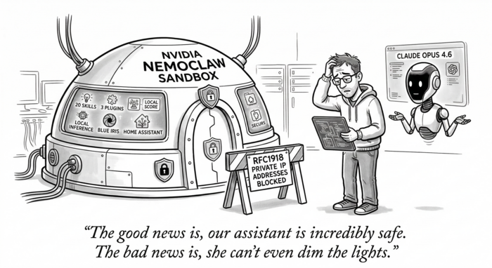
Illustration by NanoBanana</em></p>

<p>A vacant one-bedroom on March 1st and an idle H100 at 2 AM share the same brutal economic truth: the revenue from that moment is gone forever. The rent you didn’t collect last month and the compute you didn’t sell last hour are both inventory that perished on the shelf. Fixed costs — the mortgage payment, the power bill for the cooling system — don’t care whether anyone showed up.</p>

<p>This isn’t a cute analogy. It’s the same problem, and increasingly, both industries are arriving at the same solutions.</p>

<h2 id="two-markets-one-structure">Two Markets, One Structure</h2>

<p>The parallels between GPU cloud compute and multifamily housing run deeper than you might expect.</p>

<p><strong>Both sell time-bound capacity.</strong> An apartment is really a bundle of unit-months. A cloud GPU is a bundle of GPU-hours. Neither can be warehoused. If a 300-unit property runs at 93% occupancy, those 21 vacant unit-months each month are revenue that will never come back. If a rack of NVIDIA B200s — representing millions of dollars in upfront hardware cost — sits at 40% utilization, the idle hours are burning cash at a staggering rate.</p>

<p><strong>Both face agonizing supply lags.</strong> New apartment construction takes 18 to 24 months from groundbreaking to first lease-up. New GPU fabrication capacity takes two to three years to come online. The result in both cases is boom-and-bust cycles where supply overshoots or undershoots demand by the time it arrives.</p>

<p><strong>Both experience demand volatility.</strong> Multifamily leasing follows seasonal patterns — summer peaks, winter troughs — overlaid with macro cycles of job growth and migration. GPU demand spikes around major model training runs, new chip launches, and shifts between training and inference workloads. The amplitude is different (GPU demand can move 10x overnight when a new foundation model drops), but the shape is the same.</p>

<p><strong>Both use price as the primary balancing mechanism.</strong> And this is where the convergence gets interesting.</p>

<h2 id="the-data-tells-the-same-story">The Data Tells the Same Story</h2>

<p>On the GPU side, the pattern is vivid. 3Fourteen Research tracks real-time on-demand GPU availability across cloud providers, and their data shows wild cyclicality. Through late 2023 and early 2024, on-demand availability for H100s was near zero — you simply couldn’t get one. By mid-2025, supply caught up: H100 and GH200 availability surged to 80–90% as new capacity came online. Then Blackwell arrived, demand exploded again, and by early 2026, availability for the newest GPUs collapsed back toward zero. The chart looks less like a steady-state market and more like a seismograph.</p>

<p><img src="/images/perishable-inventory/gpu-availability-3fourteen.jpeg" alt="3Fourteen Research GPU on-demand availability tracker showing percent of minutes in hour with availability for A100, H100, GH200, and B200 GPUs from August 2023 to February 2026" />
<em>
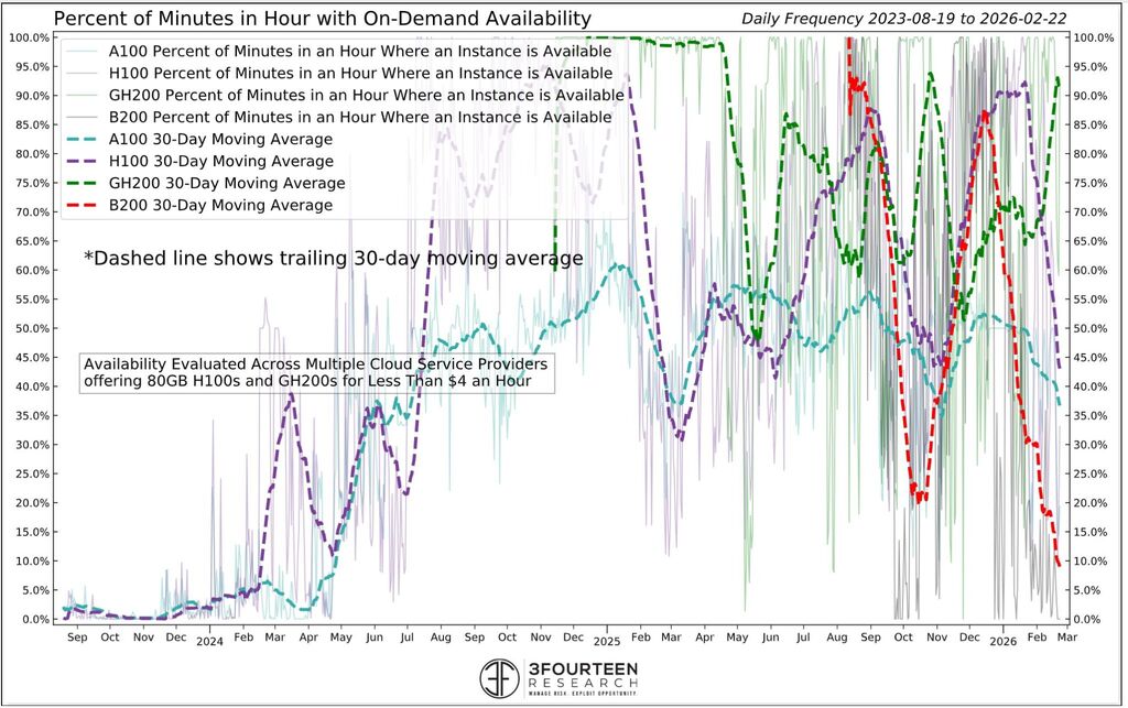
GPU on-demand availability across cloud providers, Aug 2023 – Feb 2026. Note the wild swings from near-zero to 90%+ and back. Source: <a href="https://www.3fourteenresearch.com/">3Fourteen Research</a></em></p>

<p>The multifamily market tells a remarkably similar story, just on a slower timescale. Developers delivered nearly 600,000 new apartment units in 2024 — the most since 1974 — with the Sun Belt absorbing a disproportionate share. Charlotte grew its apartment stock by nearly 8% in a single year; Austin exceeded 10%. The predictable result: occupancy softened, and advertised rents in Sun Belt markets turned negative — Austin down over 3%, Phoenix down over 4%, Denver nearly 2%. It was the apartment equivalent of the mid-2025 GPU glut — supply finally arriving just as the market had already repriced expectations.</p>

<p><img src="/images/perishable-inventory/multifamily-occupancy-chart.png" alt="U.S. multifamily and rental occupancy rates quarterly from 2018 to 2025, showing pandemic tightening, record low vacancy in 2022, supply wave impact in 2023-2024, and early recovery in 2025" />
<em>
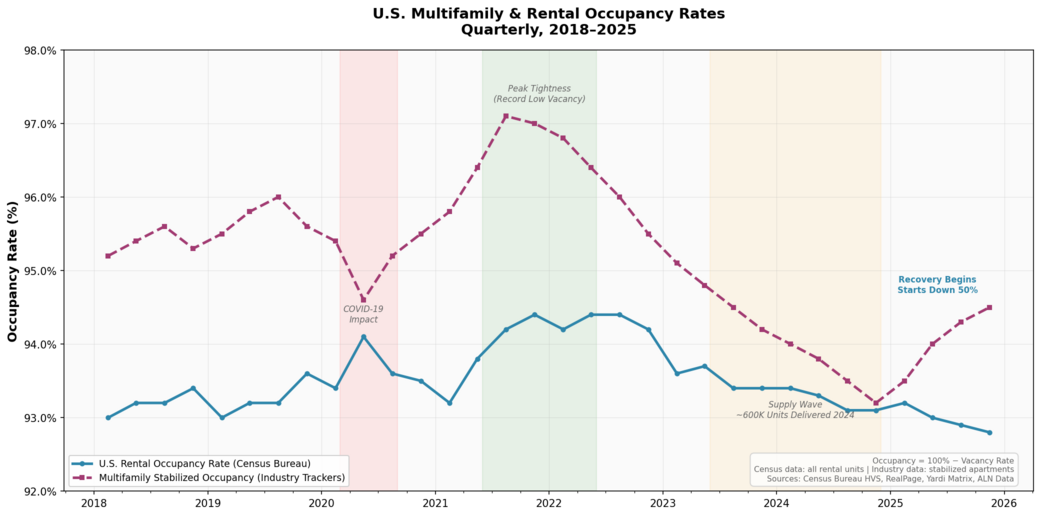
U.S. rental and multifamily stabilized occupancy rates, 2018–2025. The same boom-bust cycle plays out — just measured in quarters instead of minutes. Sources: Census Bureau HVS, RealPage, Yardi Matrix, ALN Data</em></p>

<p>But here’s the parallel that matters most: both markets are now past peak supply. Multifamily construction starts have fallen nearly 50% from their cycle high, and occupancy is recovering. GPU availability for the latest Blackwell chips is back to near-zero as demand from hyperscalers, enterprises, and AI startups overwhelms everything NVIDIA and its partners can ship. In both cases, the clock resets and the scarcity cycle begins again.</p>

<h2 id="the-revenue-management-convergence">The Revenue Management Convergence</h2>

<p>Faced with the same core problem — perishable inventory with volatile demand — both industries have converged on the same solution: algorithmic revenue management.</p>

<p>Multifamily operators now use platforms like Yardi Revenue IQ, RealPage, and newer entrants to dynamically price every unit based on real-time occupancy, seasonal patterns, local comps, and lease expiration curves. The goal isn’t to maximize the rent on any single unit; it’s to optimize total revenue across the entire portfolio, balancing occupancy against rate. A property might accept a lower rent to avoid a vacancy that would cost more in lost revenue than the discount.</p>

<p>GPU cloud providers have arrived at the same logic through a different door. Reserved instances function like long-term leases — a commitment discount in exchange for guaranteed occupancy. Spot pricing is the equivalent of last-minute apartment deals: deeply discounted, but you might get evicted (preempted) if someone pays full price. On-demand pricing is the walk-in rate, the month-to-month lease — maximum flexibility, maximum cost. The pricing tiers map almost perfectly.</p>

<p>Both are playing the same game: control demand through price inflection to maximize yield on a finite, time-sensitive asset.</p>

<h2 id="where-the-analogy-breaks">Where the Analogy Breaks</h2>

<p>The comparison isn’t perfect. GPU workloads can materialize and vanish in seconds; tenants sign 12-month leases that provide a revenue floor multifamily operators can plan around. A single customer announcement — say, a hyperscaler deciding to pre-train a new frontier model — can absorb thousands of GPUs overnight in a way that has no apartment-market equivalent.</p>

<p>And GPU supply has a flexibility lever that apartments lack: software. Multi-tenancy, fractional GPUs, and workload scheduling can effectively expand capacity without building anything new. You can’t split a one-bedroom into two half-bedrooms (legally, at least).</p>

<h2 id="the-lesson">The Lesson</h2>

<p>But these differences are matters of degree, not kind. Both industries are learning the same fundamental lesson: when your inventory perishes every hour — or every month — the management of utilization <em>is</em> the business. The building is not the product. The GPU is not the product. The <em>occupied hour</em> is the product.</p>

<p>Whether you’re running a 300-unit apartment complex or a 10,000-GPU cluster, the playbook is converging: forecast demand, price dynamically, minimize vacancy, and accept that the real enemy is always the clock.</p>

<hr />

<p><em>Sources: <a href="https://www.3fourteenresearch.com/">3Fourteen Research</a> GPU availability tracker · <a href="https://247wallst.com/investing/2026/03/15/nvidia-gpu-availability-near-zero-ai-compute-demand-off-the-charts/">24/7 Wall St.</a> on near-zero GPU availability · <a href="https://www.ciodive.com/news/cloud-ai-data-center-first-quarter-spending-spike/751199/">CIO Dive</a> on data center capex · <a href="https://www.cbre.com/insights/books/us-real-estate-market-outlook-2025/multifamily">CBRE U.S. Multifamily Outlook</a> · <a href="https://www.cushmanwakefield.com/en/united-states/insights/us-marketbeats/us-multifamily-marketbeat">Cushman &amp; Wakefield U.S. Multifamily MarketBeat</a> · Census Bureau <a href="https://fred.stlouisfed.org/series/RRVRUSQ156N">Housing Vacancies &amp; Homeownership</a> via FRED</em></p>]]></content><author><name>Jim Smith</name></author><category term="AI Strategy" /><category term="gpu" /><category term="data-centers" /><category term="multifamily" /><category term="revenue-management" /><category term="occupancy" /><category term="analysis" /><summary type="html"><![CDATA[Both industries sell time-bound capacity. Both are converging on the same playbook.]]></summary></entry><entry><title type="html">Running MiniMax-M2.5 on a Single RTX 6000 Blackwell: 68 Tokens/s with 64K Context</title><link href="https://joshua8.ai/minimax-m25-rtx-6000-blackwell-sglang-guide/" rel="alternate" type="text/html" title="Running MiniMax-M2.5 on a Single RTX 6000 Blackwell: 68 Tokens/s with 64K Context" /><published>2026-02-28T00:00:00+00:00</published><updated>2026-02-28T00:00:00+00:00</updated><id>https://joshua8.ai/minimax-m25-rtx-6000-blackwell-sglang-guide</id><content type="html" xml:base="https://joshua8.ai/minimax-m25-rtx-6000-blackwell-sglang-guide/"><![CDATA[<p>MiniMax-M2.5 is a 139B parameter mixture-of-experts model with only 10B active parameters per token, making it surprisingly efficient for its size. Using the REAP NVFP4 quantization from lukealonso, you can run it on a single NVIDIA RTX PRO 6000 Blackwell GPU with 96 GB of VRAM — and get a very usable 68 tokens per second with a 64K token context window.</p>

<p>Here’s exactly how to do it.</p>

<h2 id="the-stack">The Stack</h2>

<ul>
  <li><strong>Model:</strong> lukealonso/MiniMax-M2.5-REAP-139B-A10B-NVFP4</li>
  <li><strong>Inference engine:</strong> SGLang v0.5.8.post1</li>
  <li><strong>Docker image:</strong> lmsysorg/sglang:v0.5.8.post1-cu130</li>
  <li><strong>GPU:</strong> NVIDIA RTX PRO 6000 Blackwell (96 GB)</li>
</ul>

<h2 id="why-sglang-and-not-vllm">Why SGLang and Not vLLM?</h2>

<p>I tried vLLM first — versions 0.15.1, 0.16.0, and the cu130 nightly. All three crash with a CUDA illegal memory access in the MoE gate layer during inference. The model loads fine, the server starts, but the first request kills the engine. Both the CUTLASS and Marlin GEMM backends hit the same error. I filed this as a bug (vllm-project/vllm#35566).</p>

<p>SGLang’s FlashInfer-based MoE kernels handle the NVFP4 checkpoint without issues on Blackwell.</p>

<h2 id="the-docker-compose-file">The Docker Compose File</h2>

<div class="language-yaml highlighter-rouge"><div class="highlight"><pre class="highlight"><code><span class="na">services</span><span class="pi">:</span>
  <span class="na">sglang</span><span class="pi">:</span>
    <span class="na">image</span><span class="pi">:</span> <span class="s">lmsysorg/sglang:v0.5.8.post1-cu130</span>
    <span class="na">container_name</span><span class="pi">:</span> <span class="s">sglang-minimax-reap</span>
    <span class="na">runtime</span><span class="pi">:</span> <span class="s">nvidia</span>
    <span class="na">shm_size</span><span class="pi">:</span> <span class="s2">"</span><span class="s">1g"</span>
    <span class="na">ports</span><span class="pi">:</span>
      <span class="pi">-</span> <span class="s2">"</span><span class="s">8000:8000"</span>
    <span class="na">volumes</span><span class="pi">:</span>
      <span class="pi">-</span> <span class="s">~/.cache/huggingface:/root/.cache/huggingface</span>
    <span class="na">environment</span><span class="pi">:</span>
      <span class="pi">-</span> <span class="s">CUDA_VISIBLE_DEVICES=0</span>
      <span class="pi">-</span> <span class="s">LD_LIBRARY_PATH=/lib/x86_64-linux-gnu</span>
    <span class="na">command</span><span class="pi">:</span>
      <span class="pi">-</span> <span class="s">python3</span>
      <span class="pi">-</span> <span class="s">-m</span>
      <span class="pi">-</span> <span class="s">sglang.launch_server</span>
      <span class="pi">-</span> <span class="s">--model</span>
      <span class="pi">-</span> <span class="s">lukealonso/MiniMax-M2.5-REAP-139B-A10B-NVFP4</span>
      <span class="pi">-</span> <span class="s">--served-model-name</span>
      <span class="pi">-</span> <span class="s">minimax-m2.5-reap-nvfp4</span>
      <span class="pi">-</span> <span class="s">--reasoning-parser</span>
      <span class="pi">-</span> <span class="s">minimax</span>
      <span class="pi">-</span> <span class="s">--tool-call-parser</span>
      <span class="pi">-</span> <span class="s">minimax-m2</span>
      <span class="pi">-</span> <span class="s">--trust-remote-code</span>
      <span class="pi">-</span> <span class="s">--tp</span>
      <span class="pi">-</span> <span class="s2">"</span><span class="s">1"</span>
      <span class="pi">-</span> <span class="s">--mem-fraction-static</span>
      <span class="pi">-</span> <span class="s2">"</span><span class="s">0.95"</span>
      <span class="pi">-</span> <span class="s">--max-running-requests</span>
      <span class="pi">-</span> <span class="s2">"</span><span class="s">32"</span>
      <span class="pi">-</span> <span class="s">--context-length</span>
      <span class="pi">-</span> <span class="s2">"</span><span class="s">65536"</span>
      <span class="pi">-</span> <span class="s">--quantization</span>
      <span class="pi">-</span> <span class="s">modelopt_fp4</span>
      <span class="pi">-</span> <span class="s">--attention-backend</span>
      <span class="pi">-</span> <span class="s">flashinfer</span>
      <span class="pi">-</span> <span class="s">--moe-runner-backend</span>
      <span class="pi">-</span> <span class="s">flashinfer_cutlass</span>
      <span class="pi">-</span> <span class="s">--kv-cache-dtype</span>
      <span class="pi">-</span> <span class="s">fp8_e5m2</span>
      <span class="pi">-</span> <span class="s">--enable-flashinfer-allreduce-fusion</span>
      <span class="pi">-</span> <span class="s">--host</span>
      <span class="pi">-</span> <span class="s2">"</span><span class="s">0.0.0.0"</span>
      <span class="pi">-</span> <span class="s">--port</span>
      <span class="pi">-</span> <span class="s2">"</span><span class="s">8000"</span>
    <span class="na">deploy</span><span class="pi">:</span>
      <span class="na">resources</span><span class="pi">:</span>
        <span class="na">reservations</span><span class="pi">:</span>
          <span class="na">devices</span><span class="pi">:</span>
            <span class="pi">-</span> <span class="na">driver</span><span class="pi">:</span> <span class="s">nvidia</span>
              <span class="na">count</span><span class="pi">:</span> <span class="s">all</span>
              <span class="na">capabilities</span><span class="pi">:</span> <span class="pi">[</span><span class="nv">gpu</span><span class="pi">]</span>
    <span class="na">restart</span><span class="pi">:</span> <span class="s">unless-stopped</span>
</code></pre></div></div>

<p>Run <code class="language-plaintext highlighter-rouge">docker compose up -d</code> and wait about two minutes for the model to load.</p>

<h2 id="two-key-settings">Two Key Settings</h2>

<p><strong>fp8 KV cache is essential.</strong> The model card recommends bf16 for the KV cache, but that only gives you about 33K tokens of capacity on 96 GB. Switching to <code class="language-plaintext highlighter-rouge">--kv-cache-dtype fp8_e5m2</code> doubles it to 67K tokens, which is enough to actually use a 65K context window. In my testing, output quality was not noticeably affected.</p>

<p><strong>Set memory fraction to 0.95.</strong> The default 0.85-0.88 range doesn’t leave enough room for the KV cache after the model’s 81.6 GB of weights are loaded. At 0.95, you get about 9 GB for KV cache, CUDA graphs, and overhead.</p>

<h2 id="performance">Performance</h2>

<p>I generated six 1000+ word stories and measured throughput:</p>

<table>
  <thead>
    <tr>
      <th>Prompt</th>
      <th style="text-align: right">Tokens</th>
      <th style="text-align: right">Time</th>
      <th style="text-align: right">Tokens/s</th>
    </tr>
  </thead>
  <tbody>
    <tr>
      <td>Elephant story</td>
      <td style="text-align: right">1,364</td>
      <td style="text-align: right">20.1s</td>
      <td style="text-align: right">67.9</td>
    </tr>
    <tr>
      <td>Fox story</td>
      <td style="text-align: right">1,580</td>
      <td style="text-align: right">23.1s</td>
      <td style="text-align: right">68.3</td>
    </tr>
    <tr>
      <td>Zebra story</td>
      <td style="text-align: right">1,334</td>
      <td style="text-align: right">19.3s</td>
      <td style="text-align: right">69.1</td>
    </tr>
    <tr>
      <td>Dolphin story</td>
      <td style="text-align: right">1,205</td>
      <td style="text-align: right">17.7s</td>
      <td style="text-align: right">67.9</td>
    </tr>
    <tr>
      <td>Owl story</td>
      <td style="text-align: right">1,248</td>
      <td style="text-align: right">18.0s</td>
      <td style="text-align: right">69.1</td>
    </tr>
    <tr>
      <td>Wolf story</td>
      <td style="text-align: right">1,328</td>
      <td style="text-align: right">19.1s</td>
      <td style="text-align: right">69.4</td>
    </tr>
  </tbody>
</table>

<p>Consistent 68-69 tokens/s on short-context generation. This is well above the 15-30 t/s some early reports suggested for this model on Blackwell. Long-context workloads (above 32K input tokens) will be slower, as expected for single-GPU MoE inference.</p>

<p>The model supports both reasoning (chain-of-thought in <code class="language-plaintext highlighter-rouge">reasoning_content</code>) and tool calling out of the box through SGLang’s OpenAI-compatible API at <code class="language-plaintext highlighter-rouge">http://localhost:8000/v1/chat/completions</code>.</p>]]></content><author><name>Jim Smith</name></author><category term="AI Technology" /><category term="sglang" /><category term="minimax" /><category term="blackwell" /><category term="rtx-6000" /><category term="inference" /><category term="local-llm" /><category term="moe" /><summary type="html"><![CDATA[How to run the 139B parameter MiniMax-M2.5 model on a single NVIDIA RTX PRO 6000 Blackwell GPU using SGLang, achieving 68 tokens/s with 64K context.]]></summary></entry></feed>